WIXLIB

Technical PaperData Modeling Considerations in Hadoopand HiveClark Bradley, Ralph Hollinshead, Scott Kraus, Jason Lefler, Roshan TaheriOctober 2013

Table of ContentsIntroduction . 2Understanding HDFS and Hive . 2Project Environment . 4Hardware . 4Software . 5The Hadoop Cluster . 7The Client Server . 9The RDBMS Server. 9Data Environment Setup . 9Approach for Our Experiments . 13Results . 14Experiment 1: Flat File versus Star Schema . 14Experiment 2: Compressed Sequence Files . 16Experiment 3: Indexes. 17Experiment 4: Partitioning . 19Experiment 5: Impala . 21Interpretation of Results . 22Conclusions . 24Appendix . 25Queries Used in Testing Flat Tables . 25References . 26

Data Modeling Considerations in Hadoop and HiveIntroductionIt would be an understatement to say that there is a lot of buzz these days about big data. Because of the proliferation ofnew data sources such as machine sensor data, medical images, financial data, retail sales data, radio frequencyidentification, and web tracking data, we are challenged to decipher trends and make sense of data that is orders ofmagnitude larger than ever before. Almost every day, we see another article on the role that big data plays in improvingprofitability, increasing productivity, solving difficult scientific questions, as well as many other areas where big data issolving problems and helping us make better decisions. One of the technologies most often associated with the era of bigdata is Apache Hadoop.Although there is much technical information about Hadoop, there is not much information about how to effectivelystructure data in a Hadoop environment. Even though the nature of parallel processing and the MapReduce systemprovide an optimal environment for processing big data quickly, the structure of the data itself plays a key role. Asopposed to relational data modeling, structuring data in the Hadoop Distributed File System (HDFS) is a relatively newdomain. In this paper, we explore the techniques used for data modeling in a Hadoop environment. Specifically, the intentof the experiments described in this paper was to determine the best structure and physical modeling techniques forstoring data in a Hadoop cluster using Apache Hive to enable efficient data access. Although other software interacts withHadoop, our experiments focused on Hive. The Hive infrastructure is most suitable for traditional data warehousing-typeapplications. We do not cover Apache HBase, another type of Hadoop database, which uses a different style of modelingdata and different use cases for accessing the data.In this paper, we explore a data partition strategy and investigate the role indexing, data types, files types, and other dataarchitecture decisions play in designing data structures in Hive. To test the different data structures, we focused on typicalqueries used for analyzing web traffic data. These included web analyses such as counts of visitors, most referring sites,and other typical business questions used with weblog data.The primary measure for selecting the optimal structure for data in Hive is based on the performance of web analysisqueries. For comparison purposes, we measured the performance in Hive and the performance in an RDBMS. The reasonfor this comparison is to better understand how the techniques that we are familiar with using in an RDBMS work in theHive environment. We explored techniques such as storing data as a compressed sequence file in Hive that are particularto the Hive architecture.Through these experiments, we attempted to show that how data is structured (in effect, data modeling) is just asimportant in a big data environment as it is in the traditional database world.Understanding HDFS and HiveSimilar to massively parallel processing (MPP) databases, the power of Hadoop is in the parallel access to data that canreside on a single node or on thousands of nodes. In general, MapReduce provides the mechanism that enables accessto each of the nodes in the cluster. Within the Hadoop framework, Hive provides the ability to create and query data on alarge scale with a familiar SQL-based language called HiveQL. It is important to note that in these experiments, we strictlyused Hive within the Hadoop environment. For our tests, we simulated a typical data warehouse-type workload wheredata is loaded in batch, and then queries are executed to answer strategic (not operational) business questions.2

Technical PaperAccording to the Apache Software Foundation, here is the definition of Hive:“Hive is a data warehouse system for Hadoop that facilitates easy data summarization, ad-hoc queries, and theanalysis of large datasets stored in Hadoop compatible file systems. Hive provides a mechanism to project structureonto this data and query the data using a SQL-like language called HiveQL. At the same time this language alsoallows traditional map/reduce programmers to plug in their custom mappers and reducers when it is inconvenient orinefficient to express this logic in HiveQL.”To demonstrate how to structure data in Hadoop, our examples used the Hive environment. Using the SAS/ACCESSengine, we were able to run our test queries through the SAS interface, which is executed in the Hive environment withinour Hadoop cluster. In addition, we performed a cursory examination of Impala, the “SQL on top of Hadoop” tool offeredby Cloudera.All queries executed through SAS/ACCESS to Hadoop were submitted via the Hive environment and were translated intoMapReduce jobs. Although it is beyond the scope of this paper to detail the inner-workings of MapReduce, it is importantto understand how data is stored in HDFS when using Hive to better understand how we should structure our tables inHadoop. By gaining some understanding in this area, we are able to appreciate the effect data modeling techniques havein HDFS.In general, all data stored in HDFS is broken into blocks of data. We used Cloudera’s distribution of version 4.2 of Hadoopfor these experiments. The default size of each data block in Cloudera Hadoop 4.2 is 128 MB. As shown in Figure 1, thesame blocks of data were replicated across multiple nodes to provide reliability if a node failed, and also to increase theperformance during MapReduce jobs. Each block of data is replicated three times by default in the Hadoop environment.The NameNode in the Hadoop cluster serves as the metadata repository that describes where blocks of data are locatedfor each file stored in HDFS.Figure 1: HDFS Data Storage[5]

Data Modeling Considerations in Hadoop and HiveAt a higher level, when a table is created through Hive, a directory is created in HDFS on each node that represents thetable. Files that contain the data for the table are created on each of the nodes, and the Hive metadata keeps track ofwhere the files that make up each table are located. These files are located in a directory with the name of the table inHDFS in the /user/hive/warehouse folder by default. For example, in our tests, we created a table namedBROWSER DIM. We can use an HDFS command to see the new table located in the /user/hive/warehousedirectory. By using the command hadoop fs -ls, the contents of the browser dim directory are listed. In thisdirectory, we find a file named browser dim.csv. HDFS commands are similar to standard Linux commands.By default, Hadoop distributes the contents of the browser dim table into all of the nodes in the Hadoop cluster. Thefollowing hadoop fs –tail command lists the last kilobyte of the file listed:601235 Safari601236 Safari601237 Safari601238 Safari11111 11.1 r1211 11.1 r1021 11.1 r1021 11.2 r202111101 1.6.0 29 Macintosh1 1.6.0 29 Macintosh1 1.6.0 31 Macintosh24 1024x60024 1280x80024 1280x80024 1280x800The important takeaway is to understand at a high level how data is stored in HDFS and managed in the Hiveenvironment. The physical data modeling experiments that we performed ultimately affect how the data is stored in blocksin HDFS and in the nodes where the data is located and how the data is accessed. This is particularly true for the tests inwhich we partitioned the data using the Partition statement to redistribute the data based on the buckets or rangesdefined in the partitions.Project EnvironmentHardwareThe project hardware was designed to emulate a small-scale Hadoop cluster for testing purposes, not a large-scaleproduction environment. Our blades had only two CPUs each. Normally, Hadoop cluster nodes have more. However, thesize of the cluster and the data that we used are large enough to make conclusions about physical data modelingtechniques. As shown in Figure 2, our hardware configuration was as follows:Overall hardware configuration: 1 Dell M1000e server rack 10 Dell M610 blades Juniper EX4500 10 GbE switch4

Technical PaperBlade configuration: Intel Xeon X5667 3.07GHz processor Dell PERC H700 Integrated RAID controller Disk size: 543 GB FreeBSD iSCSI Initiator driver HP P2000 G3 iSCSI dual controller Memory: 94.4 GB Linux 2.6.32Figure 2: The Project Hardware EnvironmentSoftwareThe project software created a small-scale Hadoop cluster and included a standard RDBMS server and a client serverwith release 9.3 of Base SAS software with supporting software.

Data Modeling Considerations in Hadoop and HiveThe project software included the following components: CDH (Cloudera’s Distribution Including Apache Hadoop) version 4.2.1oApache Hadoop 2.0.0oApache Hive 0.10.0oHUE (Hadoop User Experience) 2.2.0oImpala 1.0oApache MapReduce 0.20.2oApache Oozie 3.3.0oApache ZooKeeper 3.4.5 Apache Sqoop 1.4.2 Base SAS 9.3 A major relational database6

Technical PaperFigure 3: The HDFS ArchitectureThe Hadoop ClusterThe Hadoop cluster can logically be divided into two areas: HDFS, which stores the data, and MapReduce, whichprocesses all of the computations on the data (with the exception of a few tests where we used Impala).The NameNode on nodes 1 and 2 and the JobTracker on node 1 (in the next figure) serve as the master nodes. The othersix nodes are acting as slaves.[1]Figure 3 shows the daemon processes of the HDFS architecture, which consist of two NameNodes, seven DataNodes,two Failover Controllers, three Journal Nodes, one HTTP FS, one Balancer, and one Hive Metastore. The NameNodelocated on blade Node 1 is designated as the active NameNode. The NameNode on Node 2 is serving as the standby.Only one NameNode can be active at a time. It is responsible for controlling the data storage for the cluster. When theNameNode on Node 2 is active, the DataNode on Node 2 is disabled in accordance with accepted HDFS procedure. TheDataNodes act as instructed by the active NameNode to coordinate the storage of data. The Failover Controllers aredaemons that monitor the NameNodes in a high-availability environment. They are responsible for updating theZooKeeper session information and initiating state transitions if the health of the associated NameNode wavers.[2] The

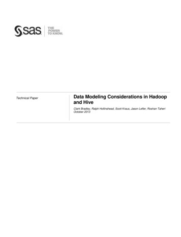
Data Modeling Considerations in Hadoop and HiveJournalNodes are written to by the active NameNode whenever it performs any modifications in the cluster. The standbyNameNode has access to all of the modifications if it needs to transition to an active state.[3] The HTTP FS provides theinterface between the operating system on the server and HDFS.[4] The Balancer utility distributes the data blocks acrossthe nodes evenly.[5] The Hive Metastore contains the information about the Hive tables and partitions in the cluster.[6]Figure 4 depicts the system’s MapReduce architecture. The JobTracker is responsible for controlling the parallelprocessing of the MapReduce functionality. The TaskTrackers act as instructed by the JobTracker to process theMapReduce jobs.[1]8