Transcription
Lecture 13Network FlowSupplemental reading in CLRS: Sections 26.1 and 26.2When we concerned ourselves with shortest paths and minimum spanning trees, we interpreted theedge weights of an undirected graph as distances. In this lecture, we will ask a question of a differentsort. We start with a directed weighted graph G with two distinguished vertices s (the source) andt (the sink). We interpret the edges as unidirectional water pipes, with an edge’s capacity indicatedby its weight. The maximum flow problem then asks, how can one route as much water as possiblefrom s to t?To formulate the problem precisely, let’s make some definitions.Definition. A flow network is a directed graph G (V , E) with distinguished vertices s (the source)and t (the sink), in which each edge (u, v) E has a nonnegative capacity c(u, v). We require that Enever contain both (u, v) and (v, u) for any pair of vertices u, v (so in particular, there are no loops).Also, if u, v V with (u, v) 6 E, then we define c(u, v) to be zero. (See Figure 13.1).In these notes, we will always assume that our flow networks are finite. Otherwise, it would bequite difficult to run computer algorithms on them.Definition. Given a flow network G (V , E), a flow in G is a function f : V V R satisfying1. Capacity constraint: 0 f (u, v) c(u, v) for each u, v V1216s2049t741314Figure 13.1. A flow network.
2. Flow conservation: for each u V \ { s, t}, we have1Xf (v, u) v V Xf (u, v) .v V{z}flow into u {z}flow out of uIn the case that flow conservation is satisfied, one can prove (and it’s easy to believe) that the net flowout of s equals the net flow into t. This quantity is called the flow value, or simply the magnitude,of f . We writeXXXX f f (s, v) f (v, s) f (v, t) f (t, v). {z}v Vv Vv Vv Vflow valueNote that the definition of a flow makes sense even when G is allowed to contain both an edgeand its reversal (and therefore is not truly a flow network). This will be important in §13.1.1 whenwe discuss augmenting paths.13.1The Ford–Fulkerson AlgorithmThe Ford–Fulkerson algorithm is an elegant solution to the maximum flow problem. Fundamentally, it works like this:12while there is a path from s to t that can hold more water doPush more water through that pathTwo notes about this algorithm: The notion of “a path from s to t that can hold more water” is made precise by the notion of anaugmenting path, which we define in §13.1.1. The Ford–Fulkerson algorithm is essentially a greedy algorithm. If there are multiple possibleaugmenting paths, the decision of which path to use in line 2 is completely arbitrary.2 Thus,like any terminating greedy algorithm, the Ford–Fulkerson algorithm will find a locally optimal solution; it remains to show that the local optimum is also a global optimum. This is donein §13.2.13.1.1Residual Networks and Augmenting PathsThe Ford–Fulkerson algorithm begins with a flow f (initially the zero flow) and successively improvesf by pushing more water along some path p from s to t. Thus, given the current flow f , we need1 In order for a flow of water to be sustainable for long periods of time, there cannot exist an accumulation of excesswater anywhere in the pipe network. Likewise, the amount of water flowing into each node must at least be sufficient tosupply all the outgoing connections promised by that node. Thus, the amount of water entering each node must equal theamount of water flowing out. In other words, the net flow into each vertex (other than the source and the sink) must bezero.2 There are countless different versions of the Ford–Fulkerson algorithm, which differ from each other in the heuristicfor choosing which augmenting path to use. Different situations (in which we have some prior information about thenature of G) may call for different heuristics.Lec 13 – pg. 2 of 11
a way to tell how much more water a given path p can carry. To start, note that a chain is only asstrong as its weakest link: if p 〈v0 , . . . , vn 〉, thenµ¶amount of additional waterthat can flow through p¶µamount of additional water that.1 i n can flow directly from v i 1 to v imin All we have to know now is how much additional water can flow directly between a given pair ofvertices u, v. If (u, v) E, then clearly the flow from u to v can be increased by up to c(u, v) f (u, v).Next, if (v, u) E (and therefore (u, v) 6 E, since G is a flow network), then we can simulate anincreased flow from u to v by decreasing the throughput of the edge (v, u) by as much as f (v, u).Finally, if neither (u, v) nor (v, u) is in E, then no water can flow directly from u to v. Thus, we definethe residual capacity between u and v (with respect to f ) to be c(u, v) f (u, v) if (u, v) Ec f (u, v) f (v, u)(13.1)if (v, u) E 0otherwise.When drawing flows in flow networks, it is customary to label an edge (u, v) with both the capacityc(u, v) and the throughput f (u, v), as in Figure 13.2.Next, we construct a directed graph G f , called the residual network of f , which has the samevertices as G, and has an edge from u to v if and only if c f (u, v) is positive. (See Figure 13.2.) Theweight of such an edge (u, v) is c f (u, v). Keep in mind that c f (u, v) and c f (v, u) may both be positivefor some pairs of vertices u, v. Thus, the residual network of f is in general not a flow network.Equipped with the notion of a residual network, we define an augmenting path to be a pathfrom s to t in G f . If p is such a path, then by virtue of our above discussion, we can perturb the flowf at the edges of p so as to increase the flow value by c f (p), wherec f (p) min c f (u, v).(u,v) p(13.2)The way to do this is as follows. Given a path p, we might as well assume that p is a simple path.3In particular, p will never contain a given edge more than once, and will never contain both an edgeand its reversal. We can then define a new flow f 0 in the residual network (even though the residualnetwork is not a flow network) by setting(f 0 (u, v) c f (p)if (u, v) p0otherwise.Exercise 13.1. Show that f 0 is a flow in G f , and show that its magnitude is c f (p). Finally, we can “augment” f by f 0 , obtaining a new flow f f 0 whose magnitude is f f 0 3 Recall that a simple path is a path which does not contain any cycles. If p is not simple, we can always pare p down toa simple path by deleting some of its edges (see Exercise B.4-2 of CLRS, although the claim I just made is a bit stronger).Doing so will never decrease the residual capacity of p (just look at (13.2)).Lec 13 – pg. 3 of 11
4Residual Network1255411s351415t7845311Augmented Flow12/1211/1619/201/4s0/97/7t12/134/411/14New Residual Network121511s19319t71241311Figure 13.2. We begin with a flow network G and a flow f : the label of an edge (u, v) is “a/b,” where a f (u, v) is the flowthrough the edge and b c(u, v) is the capacity of the edge. Next, we highlight an augmenting path p of capacity 4 in theresidual network G f . Next, we augment f by the augmenting path p. Finally, we obtain a new residual network in whichthere happen to be no more augmenting paths. Thus, our new flow is a maximum flow.Lec 13 – pg. 4 of 11
f c f (p). It is defined by4¡0 f f (u, v) f (u, v) c f (p)f (u, v) c f (p) f (u, v)if (u, v) p and (u, v) Eif (v, u) p and (u, v) Eotherwise.Lemma 13.1 (CLRS Lemma 26.1). Let f be a flow in the flow network G (V , E) and let f 0 be a flowin the residual network G f . Let f f 0 be the augmentation of f by f 0 , as described in (13.3). Then f f 0 f f 0 .Proof sketch. First, we show that f f 0 obeys the capacity constraint for each edge in E and obeysflow conservationfor eachvertexin V \ { s, t}. Thus, f f 0 is truly a flow in G. Next, we obtain the identity f f 0 f f 0 by simply expanding the left-hand side and rearranging terms in thesummation.13.1.2Pseudocode Implementation of the Ford–Fulkerson AlgorithmNow that we have laid out the necessary conceptual machinery, let’s give more detailed pseudocodefor the Ford–Fulkerson algorithm.Algorithm: F ORD –F ULKERSON(G)1B Initialize flow f to zero2for each edge (u, v) E do(u, v). f 0B The following line runs a graph search algorithm (such as BFS or DFS) to find apath from s to t in G fwhile there exists a path p : s t in G f do ªc f (p) min c f (u, v) : (u, v) pfor each edge (u, v) p doB Because (u, v) G f , it must be the case that either (u, v) E or (v, u) E.B And since G is a flow network, the “or” is exclusive: (u, v) E xor (v, u) E.if (u, v) E then(u, v). f (u, v). f c f (p)else(v, u). f (v, u). f c f (p)345678910111213 For more information about breath-first and depth-first searches, see Sections 22.2 and 22.3 of CLRS.Here, we use the notation (u, v). f synonymously with f (u, v); though, the notation (u, v). f suggestsa convenient implementation decision in which we attach the value of f (u, v) as satellite data to the4 In a more general version of augmentation, we don’t require p to be a simple path; we just require that f 0 be someflow in the residual network G f . Then we define(0f (u, v) f (u, v) f 0 (u, v) f 0 (v, u)if (u, v) E0otherwise.Lec 13 – pg. 5 of 11(13.3)
edge (u, v) itself rather than storing all of f in one place. Also note that, because we often need toconsider both f (u, v) and f (v, u) at the same time, it is important that we equip each edge (u, v) Ewith a pointer to its reversal (v, u). This way, we may pass from an edge (u, v) to its reversal (v, u)without performing a costly search to find (v, u) in memory.We defer the proof of correctness to §13.2. We do show, though, that the Ford–Fulkerson algorithm halts if the edge capacities are integers.Proposition 13.2. If the edge capacities of G are integers, then the Ford–Fulkerson algorithm termi¡ nates in time O E · f , where f is the magnitude of any maximum flow for G.Proof. Each time we choose an augmenting path p, the right-hand side of (13.2) is a positive integer.Therefore, each time we augment f , the value of f increases by at least 1. Since f cannot everexceed f , it follows that lines 5–13 are repeated at most f times. Each iteration of lines 5–13takes O(E) time if we use a breadth-first or depth-first search in line 5, so the total running time of¡ F ORD –F ULKERSON is O E · f .Exercise 13.2. Show that, if the edge capacities of G are rational numbers, then the Ford–Fulkersonalgorithm eventually terminates. What sort of bound can you give on its running time?Proposition 13.3. Let G be a flow network. If all edges in G have integer capacities, then there existsa maximum flow in G in which the throughput of each edge is an integer. One such flow is given byrunning the Ford–Fulkerson algorithm on G.Proof. Run the Ford–Fulkerson algorithm on G. The residual capacity of each augmenting path p inline 5 is an integer (technically, induction is required to prove this), so the throughput of each edge isonly ever incremented by an integer. The conclusion follows if we assume that the Ford–Fulkersonalgorithm is correct. The algorithm is in fact correct, by Corollary 13.8 below.Flows in which the throughput of each edge is an integer occur frequently enough to deserve aname. We’ll call them integer flows.Perhaps surprisingly, Exercise 13.2 is not true when the edge capacities of G are allowed to bearbitrary real numbers. This is not such bad news, however: it simply says that there exists asufficiently foolish way of choosing augmenting paths so that F ORD –F ULKERSON never terminates.If we use a reasonably good heuristic (such as the shortest-path heuristic used in the Edmonds–Karpalgorithm of §13.1.3), termination is guaranteed, and the running time needn’t depend on f .13.1.3The Edmonds–Karp AlgorithmThe Edmonds–Karp algorithm is an implementation of the Ford–Fulkerson algorithm in whichthe the augmenting path p is chosen to have minimal length among all possible augmenting paths(where each edge is assigned length 1, regardless of its capacity). Thus the Edmonds–Karp algorithmcan be implemented by using a breadth-first search in line 5 of the pseudocode for F ORD –F ULKERSON.Proposition 13.4 (CLRS Theorem 26.8). In the Edmonds–Karp algorithm, the total number of aug¡ mentations is O(V E). Thus total running time is O V E 2 .Proof sketch. First one can show that the lengths of the paths p found by breadth-first search in line 5 ofF ORD –F ULKERSON are monotonically nondecreasing (this is Lemma 26.7 of CLRS).Lec 13 – pg. 6 of 11
Next, one can show that each edge e E can only be the bottleneck for p at most O(V ) times. (By“bottleneck,” we mean that e is the (or, an) edge of smallest capacity in p, so that c f (p) c f (e).) Finally, because only O(E) pairs of vertices can ever be edges in G f and because each edge canonly be the bottleneck O(V ) times, it follows that the number of augmenting paths p used inthe Edmonds–Karp algorithm is at most O(V E). Again, since each iteration of lines 5–13 of F ORD –F ULKERSON (including the breadth-first¡ search) takes time O(E), the total running time for the Edmonds–Karp algorithm is O V E 2 .The shortest-path heuristic of the Edmonds–Karp algorithm is just one possibility. Another in¡ teresting heuristic is relabel-to-front, which gives a running time of O V 3 . We won’t expect youto know the details of relabel-to-front for 6.046, but you might find it interesting to research otherheuristics on your own.13.2The Max Flow–Min Cut EquivalenceDefinition. A cut (S, T V \ S) of a flow network G is just like a cut (S, T) of the graph G in thesense of §3.3, except that we require s S and t T. Thus, any path from s to t must cross the cut(S, T). Given a flow f in G, the net flow f (S, T) across the cut (S, T) is defined asf (S, T) X Xf (u, v) u S v TX Xf (v, u).(13.4)u S v TOne way to picture this is to think of the cut (S, T) as an oriented dam in which we count waterflowing from S to T as positive and water flowing from T to S as negative. The capacity of the cut(S, T) is defined asX Xc(u, v).(13.5)c(S, T) u S v TThe motivation for this definition is that c(S, T) should represent the maximum amount of waterthat could ever possibly flow across the cut (S, T). This is explained further in Proposition 13.6.Lemma 13.5 (CLRS Lemma 26.4). Given a flow f and a cut (S, T), we havef (S, T) f .We omit the proof, which can be found in CLRS. Intuitively, this lemma is an easy consequence offlow conservation. The water leaving s cannot build up at any of the vertices in S, so it must crossover the cut (S, T) and eventually pour out into t.Proposition 13.6. Given a flow f and a cut (S, T), we havef (S, T) c(S, T).Thus, applying Lemma 13.5, we find that for any flow f and any cut (S, T), we have f c(S, T).Lec 13 – pg. 7 of 11
Proof. In (13.4), f (v, u) is always nonnegative. Moreover, we always have f (u, v) c(u, v) by thecapacity constraint. The conclusion follows.Proposition 13.6 tells us that the magnitude of a maximum flow is at most equal to the capacityof a minimum cut (i.e., a cut with minimum capacity). In fact, this bound is tight:Theorem 13.7 (Max Flow–Min Cut Equivalence). Given a flow network G and a flow f , the followingare equivalent:(i) f is a maximum flow in G.(ii) The residual network G f contains no augmenting paths.(iii) f c(S, T) for some cut (S, T) of G.If one (and therefore all) of the above conditions hold, then (S, T) is a minimum cut.Proof. Obviously (i) implies (ii), since an augmenting path in G f would give us a way to increase themagnitude of f . Also, (iii) implies (i) because no flow can have magnitude greater than c(S, T) byProposition 13.6.Finally, suppose (ii). Let S be the set of vertices u such that there exists a path su in G f .Since there are no augmenting paths, S does not contain t. Thus (S, T) is a cut of G, where T V \ S.Moreover, for any u S and any v T, the residual capacity c f (u, v) must be zero (otherwise the paths u in G f could be extended to a path s u v in G f ). Thus, glancing back at (13.1), we find thatwhenever u S and v T, we have if (u, v) E c(u, v)f (u, v) 0if (v, u) E 0 (but who cares) otherwise.Thus we havef (S, T) X Xu S v Tc(u, v) X X0 c(S, T) 0 c(S, T);u S v Tso (iii) holds. Because the magnitude of any flow is at most the capacity of any cut, f must be amaximum flow and (S, T) must be a minimum cut.Corollary 13.8. The Ford–Fulkerson algorithm is correct.Proof. When F ORD –F ULKERSON terminates, there are no augmenting paths in the residual networkGf .13.3GeneralizationsThe definition of a flow network that we laid out may seem insufficient for handling the types offlow problems that come up in practice. For example, we may want to find the maximum flow in adirected graph which sometimes contains both an edge (u, v) and its reversal (v, u). Or, we mightwant to find the maximum flow in a directed graph with multiple sources and sinks. It turns outthat both of these generalizations can easily be reduced to the original problem by performing clevergraph transformations.Lec 13 – pg. 8 of 11
uu353w53vvFigure 13.3. We can resolve the issue of E containing both an edge and its reversal by creating a new vertex and reroutingone of the old edges through that vertex.13.3.1Allowing both an edge and its reversalSuppose we have a directed weighted graph G (V , E) with distinguished vertices s and t. We wouldlike to use the Ford–Fulkerson algorithm to solve the flow problem on G, but G might not be aflow network, as E might contain both (u, v) and (v, u) for some pair of vertices u, v. The trick is toconstruct a new graph G 0 (V 0 , E 0 ) from G in the following way: Start with (V 0 , E 0 ) (V , E). For everyunordered pair of vertices { u, v} V such that both (u, v) and (v, u) are in E, add a dummy vertex wto V 0 . In E 0 , replace the edge (u, v) with edges (u, w) and (w, v), each with capacity c(u, v) (see Figure13.3). It is easy to see that solving the flow problem on G 0 is equivalent to solving the flow problemon G. But G 0 is a flow network, so we can use F ORD –F ULKERSON to solve the flow problem on G 0 .13.3.2Allowing multiple sources and sinksNext suppose we have a directed graph G (V , E) in which there are multiple sources s 1 , . . . , s k andmultiple sinks t 1 , . . . , t . Again, it makes sense to talk about the flow problem in G, but the Ford–Fulkerson algorithm does not immediately give us a way to solve the flow problem in G. The trickthis time is to add new vertices s and t to V . Then, join s to each of s 1 , . . . , s k with a directed edgeof capacity ,5 and join each of t 1 , . . . , t to t with a directed edge of capacity (see Figure 13.4).Again, it is easy to see that solving the flow problem in this new graph is equivalent to solving theflow problem in G.13.3.3Multi-commodity flowEven more generally, we might want to transport multiple types of commodities through our network simultaneously. For example, perhaps G is a road map of New Orleans and the commoditiesare emergency relief supplies (food, clothing, flashlights, gasoline. . . ) in the wake of Hurricane Katrina. In the multi-commodity flow problem, there are commodities 1, . . . , k, sources s 1 , . . . , s k , sinkst 1 , . . . , t k , and quotas (i.e., positive numbers) d 1 , . . . , d k . Each source s i needs to send d i units of commodity i to sink t i . (See Figure 13.5.) The problem is to determine whether there is a way to do sowhile still obeying flow conservation and the capacity constraint, and if so, what that way is.5 The symbol plays the role of a sentinel value representing infinity (such that x for every real number x).Depending on your programming language (and on whether you cast the edge capacities as integers or float
13.1 The Ford–Fulkerson Algorithm The Ford–Fulkerson algorithm is an elegant solution to the maximum flow problem. Fundamen-tally, it works like this: 1 while there is a path from s to t that can hold more water do 2 Push more water through t