Transcription
Computing 69, 239–263 (2002)Digital Object Identifier (DOI) 10.1007/s00607-002-1459-8Matlab Implementation of the Finite Element Method in ElasticityJ. Alberty, Kiel, C. Carstensen, Vienna, S. A. Funken, Kiel and R. Klose, KielReceived June 18, 2001; revised February 25, 2002Published online: December 5, 2002Ó Springer-Verlag 2002AbstractA short Matlab implementation for P1 and Q1 finite elements (FE) is provided for the numericalsolution of 2d and 3d problems in linear elasticity with mixed boundary conditions. Any adaptationfrom the simple model examples provided to more complex problems can easily be performed with thegiven documentation. Numerical examples with postprocessing and error estimation via an averagedstress field illustrate the new Matlab tool and its flexibility.AMS Subject Classification: 65N30, 65R20, 73C50.Keywords: Finite element method, elasticity, Matlab.1. IntroductionUnlike complex black-box commercial computer codes, this paper provides asimple and short open-box Matlab implementation of P1 and Q1 finite elements(FE) for the numerical solutions of linear elasticity problems. Instead of coveringall kinds of possible problems in one code, the proposed tool aims to be plain,easy to understand, and to modify. Therefore, only simple model examples areincluded to be adapted to whatever is needed in the spirit of [1]. We present anerror estimator which illustrates the accuracy of the numerical calculation.A different approach is realized by the company Comsol with the finite elementpackage Femlab [7]. It is a tool for the solution of partial differential equations ofmany physical phenomena, including structural mechanics. A special feature isthe comfortable mesh generator and the possibility to combine different physicalproblems. The code is written for the most part in Matlab and can be modified,except for the mesh generator and the solver for nonlinear problems. The basisfunctions in the finite element method can be chosen to be linear, quadratic, cubicor of fourth order. The solver can use adaptivity as well.The plan of our paper is as follows. The model problem, the Navier-Laméequations, with general boundary conditions is described in Sect. 2; the weakformulation and discretisation in Sect. 3. The heart of this contribution is the datarepresentation of the triangulation, the Dirichlet and Neumann boundary in
240J. Alberty et al.Sect. 4 together with the discrete space. The main steps are the assembly procedure of the stiffness matrix in Sect. 5, the right-hand side in Sect. 6, and theincorporation of the Dirichlet boundary conditions in Sect. 7. A post-processingroutine to preview the numerical solution is given in Sect. 8; in Sect. 9 an implementation of an a posteriori error estimator is presented [3], [4], [5]. Applications illustrate the usage of the new tools in Sects. 10, 11, 12, and 13 and serve asexamples for writing the user-specified Matlab routines f.m, g.m, and u d:m. Themain program is given partly in these sections and in its total in the appendices.The programs are written for Matlab 6 but adaptation for earlier versions ispossible. For a finite element calculation it is necessary to run the mainprogram with (user-specified files) coordinates.dat, elements.dat,dirichlet.dat, and neumann.dat if necessary, as well as the sub-routinesf.m, g.m, and u d:m. The graphical representation is performed with the functionshow.m and the error is estimated in aposteriori.m. All files with the codeand the data for all examples can be downloaded from www.math.tuwien.ac.at/ carsten/.2. Model ProblemThe proposed Matlab program employs the finite element method to calculatea numerical solution U which approximates the solution u to the followingd-dimensional Navier-Lamé problem (P ). Let X Rd be a bounded Lipschitzdomain with polygonal boundary C. On some closed subset CD of theboundary with positive length, we assume Dirichlet conditions while we haveNeumann boundary conditions on the (possible empty) part CN . The d components of the displacement u need not satisfy either Dirichlet- or Neumannconditions, i.e., CD and CN may overlap. Given f 2 L2 ðXÞ, M 2 L1 ðCD Þd d ,w 2 H 1 ðXÞ, and g 2 L2 ðCN Þ as well as the positive parameters k and l, seeku 2 H 1 ðXÞ withðk þ lÞðr div uÞT þ lDu ¼in X;ð1Þon CN ;on CD ;ð2Þð3Þfðk trð ðuÞÞI þ 2l ðuÞÞ n ¼ gM u¼ wwhere ðuÞ ¼ ðru þ ðruÞT Þ 2. The matrix M contains in row number j ¼ 1; . . . ; dthe entries mj1 ; . . . ; mjd (explained in Sect. 7) to model gliding geometric boundaryconditions. According to Korn’s inequality and the Lax-Milgram Lemma [2, 6],there exists a weak solution to (1)–(3) for reasonable boundary conditions in(3), i.e., there exists u 2 H 1 ðXÞ that satisfies (3) and, for all v 2 HD1 ðXÞ :¼fv 2 H 1 ðXÞ : Mv ¼ 0 on CD g,ZX ðvÞ : C ðuÞ dx ¼ZXf v dx þZg v ds:CNð4Þ
Matlab Implementation of the Finite Element Method in Elasticity241(C is the fourth-order isotropic material tensor corresponding to (1).) The weakform (4) will be relevant in the sequel and so boundary conditions are treatedcorrectly while (2) can be wrong if only some components of u on CN \ CD arefixed and so (2) holds only for some projections of both sides.3. Finite Element DiscretisationFor the implementation, problem (4) is discretised using the standard Galerkinmethod. The space H 1 ðXÞ is replaced by the finite dimensional subspace S. If whis the projection of w onto S, the discretised problem (PS ) reads: Seek uh 2 Ssuch that Muh ¼ wh on CD and, for all vh 2 S with Mvh ¼ 0 on CD ,Z ðvh Þ : C ðuh Þ dx ¼ZXf vh dx þZð5Þg vh ds:XCNLet T denote a triangulation of X specified in Sect. 4 and let N be the set of allnodes in T; set ðg1 ; . . . ; gdN Þ ¼ ðu1 e1 ; u1 e2 ; . . . ; u1 ed ; . . . ; uN e1 ; uN e2 ; . . . ; uN ed Þbe the nodal basis of the finite dimensional space S, where N is the number ofnodes of the mesh, d the dimension of the displacement vector, and uz is the scalarhat function of node z in the triangulation T, i.e., uz ðzÞ ¼ 1 and uz ðyÞ ¼ 0 for ally 2 N with y 6¼ z. Up to geometric boundary conditions (involved in Sect. 7), (5)readsZ ðgk Þ : C ðuh Þdx ¼XZf gk dx þXZFor the discrete displacement vector we have uh ¼the linear system of equationsdN ZX‘¼1 ðgk Þ : C ðg‘ Þdx U‘ ¼Xðk ¼ 1; . . . ; dN Þ:g gk dsð6ÞCNZf gk dx þXPdN‘¼1U‘ g‘ and thus (6) yieldsZg gk dsðk ¼ 1; . . . ; dN Þ: ð7ÞCNThe coefficient matrix (global stiffness matrix) A ¼ ðAk‘ Þ 2 RdN dN and the righthand side b ¼ ðbk Þ 2 RdN are defined asAk‘ ¼ZX ðgk Þ : C ðg‘ Þdxandbk ¼ZXf gk dx þZg gk ds:ð8ÞCNThe coefficient matrix is sparse, symmetric and positive semidefinite. The condition Muh ¼ wh on CD and Mvh ¼ 0 on CD will be incorporated in Sect. 7 viaLagrange multipliers.
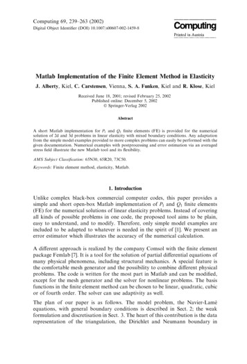
242J. Alberty et al.4. Data Representation of the Triangulation by aSupposing the domain X has a polygonalboundary C, we can cover XS regular triangulation T, i.e., X ¼ T 2T T , where the elements of T are trianglesand/or quadrilaterals for d ¼ 2 and tetrahedrons for d ¼ 3. Regular triangulationin the sense of Ciarlet [6] means that the nodes N of the mesh lie on the vertices ofthe elements, the elements of the triangulation do not overlap, no node lies on anedge of an element, and each edge E C of an element T 2 T belongs completely N , completely to C D , or completely to both.to CMatlab supports reading data from files given in ASCII format by *.dat files.Fig. 1 shows the mesh of a two dimensional example and the corresponding filecoordinates.dat, which contains the coordinates of each node. The two realnumbers per row are the x- and y-coordinates of each node.The files elements3.dat and elements4.dat contain for each triangularand quadrilateral element the node numbers of the vertices, numbered anticlockwise. See, for instance, the triangular element marked 1 in Fig. 1 which isgiven by the node numbers ð13; 3; 2Þ and not ð13; 2; 3Þ.The space S is chosen globally continuous and linear on each triangle (d ¼ 2) ortetrahedron (d ¼ 3) and bilinear on each quadrilateral element.With this space S and its corresponding nodal basis, the integrals in (8) can becalculated as a sum over all elements and a sum over all edges on CN , i.e., forj; k ¼ 1; . . . ; dN ,Ajk ¼XZT 2Tbj ¼XZT 2T ðgj Þ : C ðgk Þdx;TTf gj dx þXZE CNð9Þg gj ds:EFig. 1. Plot of triangulation and corresponding data file coordinates.datð10Þ
Matlab Implementation of the Finite Element Method in Elasticity243Fig. 2. Data files elements3.dat and elements4.datThe files neumann.dat and dirichlet.dat contain the two node numberswhich bound the corresponding edge on the boundary. In this way, the sum overE CN results in a loop over all entries in neumann.dat. The right-hand side fand g is evaluated in Sect. 6 and the Dirichlet conditions from u d:m are discussedin Sect. 7.5. Assembling the Stiffness MatrixThe local stiffness matrix is determined by the coordinates of the vertices of thecorresponding element and is calculated in the function stima3 for triangularelements, stima4 for quadrilateral elements, and stima for tetrahedral elements.Fig. 3. Data files dirichlet.dat and neumann.dat
244J. Alberty et al.Let k1 through kK be the numbers of the nodes of an element T . For a d-dimensionalproblem there are then dK basis functions with support on T , namelygpðT ;1Þ ¼ uk1 e1 ; . . . ; gpðT ;dÞ ¼ uk1 ed ;gpðT ;dKðd 1ÞÞ¼ ukK e1 ; . . . ; gpðT ;dKÞ ¼ ukK ed ;where ej is the j-th unit vector. The function ukj is the local scalar hat function ofnode kj . The function p maps the indices 1; . . . ; dK of the local numeration withrespect to T to the global numeration. The entries of the local stiffness matrix ofan element T readSTIMAðT Þk‘ ¼Z ðgpðT ;kÞ Þ : C ðgpðT ;‘Þ Þdxðk; ‘ ¼ 1; . . . ; dKÞð11ÞTand are assembled to the global stiffness matrix A. This means, the entry Apq is thesum of STIMAðT Þk‘ over all elements T with p ¼ pðT ; kÞ and q ¼ pðT ; ‘Þ, which isperformed by the following Matlab commands for the two-dimensional case fortriangles and quadrilaterals.The local stiffness matrix for each element T requires an individual discussion fortriangular, tetrahedral, and quadrilateral elements.5.1. Triangular ElementsWe consider triangular elements with the vertices ðxj ; yj ; zj Þ for j ¼ 1; 2; 3. TheVoigt representation c : H 1 ðXÞ ! L2 ðXÞ of the linear Green strain tensor reads01 01@u1 @x 11 ðuÞA ¼ @ 22 ðuÞ A:@u2 @ycðuÞ ¼ @@u2 @x þ @u1 @y2 12 ðuÞð12Þ
Matlab Implementation of the Finite Element Method in Elasticity245For r ¼ C ðuÞ we have the relation01 0r11k þ 2l@ r22 A ¼ @ k0r12101k0 11 ðuÞk þ 2l 0 A@ 22 ðuÞ A ¼: CcðuÞ:0l2 12 ðuÞð13Þand thus obtain ðvÞ : C ðuÞ ¼ r11 11 þ r22 22 þ r12 12 þ r21 21 ¼ cT ðvÞCcðuÞ: fflfflfflfflfflffl}ð14Þ¼2r12 12From (11) and relation (14) and the fact that gpðT ;kÞ etc. are affine on T it followsthatZcðgpðT ;kÞ ÞT CcðgpðT ;‘Þ Þdx ¼ jT jcðgpðT ;kÞ ÞT CcðgpðT ;‘Þ Þ:ð15ÞSTIMAðT Þk‘ ¼TLaborious but elementary calculations verifyc6Xj¼10 110 1u1u1uk1 ;x 0 uk2 ;x 0 uk3 ;x 0B . CB . CjT ¼ @ 0 uk1 ;y 0 uk2 ;y 0 uk2 ;y A@ . A ¼: R@ . Auk1 ;y uk1 ;x uk2 ;y uk2 ;x uk3 ;y uk2 ;xu6u6!uj gpðT ;jÞ0ð16Þand hence expression (15) can be written simultaneously for all indices asSTIMAðT Þ ¼ jT jRT CR:ð17ÞThe following function is a Matlab implementation of (17):This function makes use of the fact that the gradients of the scalar basis functionscan be calculated as010ruk1y21@ ruk A ¼@ y322jT jruk3y1y3y1y2x3x1x21 0x21x3 A ¼ @ x1x1y11x2y21 1001x3 A @ 10y3100 A:1ð18Þ
246J. Alberty et al.5.2. Tetrahedral ElementsThe Voigt representation c : H 1 ðXÞ3 ! L2 ðXÞ6 of the linear Green strain tensorreads1 01 11 ðuÞ@u1 @xC B 22 ðuÞ CB@u2 @yC BCBC B 33 ðuÞ CB@u @z3CC:BBcðuÞ ¼ BC¼BCB @u1 y þ @u2 x C B 2 12 ðuÞ C@ @u1 z þ @u3 x A @ 2 13 ðuÞ A@u2 z þ @u3 y2 23 ðuÞ0ð19ÞUsing the relation1 0r11k þ 2lB r22 C B kC BBB r33 C B kC BBB r12 C ¼ B 0C BB@ r13 A @ 00r230kk þ 2lk000kkk þ 2l000000l000000l0101 11 ðuÞ0CB0CCB 22 ðuÞ CCB0 CB 33 ðuÞ CC ¼: CcðuÞ; ð20ÞCB0CCB 2 12 ðuÞ CA@02 13 ðuÞ Al2 23 ðuÞwe obtain ðvÞ : C ðuÞ ¼ cT ðvÞCcðuÞ. Since again gpðT ;kÞ etc. are affine on T , (15)also holds for tetrahedral elements, but this time with C as defined in 12. Finally,we havec012X!uj gpðT ;jÞ jT ¼j¼1uk1 ;xB 0BBB 0BBuB k1 ;yB@ uk1 ;z0uk1 ;y00uk2 ;x00uk1 ;xuk1 ;z0000uk1 ;z01u1B . CC B@ . Au120uk2 ;y00uk3 ;x0uk2 ;z00uk2 ;y0uk2 ;xuk1 ;xuk2 ;z0uk1 ;y0uk2 ;z0uk3 ;y00uk4 ;x00uk4 ;yuk3 ;z000uk3 ;y0uk3 ;xuk4 ;yuk4 ;xuk2 ;xuk3 ;z0uk3 ;xuk4 ;z0uk2 ;y0uk3 ;zuk3 ;y0uk4 ;z100 CCCuk4 ;z CC0 CCCuk4 ;x Auk4 ;yð21Þand so we obtain (17), where R is the coefficient matrix on the right-hand side of(21).
Matlab Implementation of the Finite Element Method in Elasticity247The Matlab realisation of (17) for tetrahedral elements utilizes01 0ruk11B ruk C B x12 CBB@ ruk A ¼ @ y13ruk4z11x2y2z21x3y3z311x4 CCy4 Az4100B1B@000010100CC0A1ð22Þand reads as follows.5.3. Quadrilateral ElementsFinally, we consider quadrilateral elements with vertices ðx1 ; y1 Þ through ðx4 ; y4 Þ.Since T is a parallelogram, there exists an affine mappingUðn; gÞ ¼ xx2¼yy2x1y1x4y4x1y1 nx1þgy1ð23Þwhich maps ½0; 1 2 onto T . The shape functions on Tref ¼ ½0; 1 2 are defined as g1 ðn; gÞ ¼ g7 ðn; gÞ ¼ 1 ðn; gÞu;0 4 ðn; gÞu;0 0; 1 ðn; gÞu g2 ðn; gÞ ¼. g8 ðn; gÞ ¼0 4 ðn; gÞuð24Þwith 1 ðn; gÞ ¼ ð1 nÞð1u 3 ðn; gÞ ¼ ng;ugÞ; 2 ðn; gÞ ¼ nð1 gÞ;u 4 ðn; gÞ ¼ ð1 nÞg:uð25ÞThe entries of the local stiffness matrix for the element T are obtained by transforming the integral in (11) onto the reference element Tref . We use the followingabbreviation for the transpose of the gradient of the transformation.0F ¼@U1 1 ðx;yÞ@ @x@U2 1 ðx;yÞ@x1@U1 1 ðx;yÞ@yA:@U2 1 ðx;yÞ@yð26Þ
248J. Alberty et al.We notice that for the expression ðgpðT ;kÞ Þ : C ðgpðt;‘Þ Þ there are four differentpossibilities depending on the zero-components of the basis functions.first In the case we have to transform an expression of the form upðT ;iÞ0 ðx;yÞ : C upðT ;jÞ0 ðx;yÞ toone depending on the variables n; g, which results in k þ 2l 0ðru i Þ FF T ru j T :ð27Þ0l In the second case we have to transform u ðru i Þ Fl0pðT ;iÞ ðx;yÞ ðru i Þ F 0upðT ;jÞ ðx;yÞand obtain 0pðT ;iÞ ðx;yÞð28Þ: C upðT ;jÞ ðx;yÞ0and obtain 0 lF T ru j T :k 0In the fourth case we have to transform : C 0F T ru j T :k þ 2l In the third case we transform the expression uðru i Þ F 0 upðT ;iÞ ðx;yÞ0ð29Þ : C u0 pðT ;jÞ ðx;yÞand obtain kF T ru j T :00lð30ÞHence transforming the integration in (11) leads to four cases of the formZ E : ðru i ÞT ru j dx;ð31ÞTrefwhere E differs for each case and is the product of the three inner matrices in eachof (27)–(30) and i and j depend on the corresponding shape functions gk and g‘ asin (24). Note that E is constant on Tref . Hence, if we define the four matrices0R11 ¼ Z1Z0R22 ¼ Z0101Z10 j ðn; gÞ i ðn; gÞ @ u@udndg@n@n j ðn; gÞ i ðn; gÞ @ u@udndg@g@g i;j¼1;.;4 i;j¼1;.;42B1BB 2¼ B6B 1@1021B1¼ B6@ 121121211212C1CCC; ð32Þ2CA212211221121CC;1A2ð33Þ
Matlab Implementation of the Finite Element Method in ElasticityR12 ¼ RT21 ¼ Z0011 j ðn; gÞ i ðn; gÞ @ u@u1B1dndg¼ B@ 1@n4@g0i;j¼1;.;41 1Z11112491111111CC;1A1ð34Þthe following Matlab routine calculates the local stiffness matrix for quadrilateralelements:6. Assembling the Right-hand SideThe right-hand side contains the work of the volume forces f and the surfaceforces g. In this section, the assembling of the right-hand will be studied for thetwo-dimensional (as the three-dimensional case is analogous).The value of f are provided by f R:m and evaluated in the centre of gravity ðxS ; yS Þ ofT , to approximate the integral T f gk dx in (10),ZT1f gk dx kT 1 1 1x1x2x3 y1 y2 fj ðxS ; yS Þy3 withj :¼ modðk1; 2Þ þ 1;ð35Þwhere kT ¼ 6 if T is a triangle and kT ¼ 4 if T is a parallelogram. The followingMatlab commands calculate the f-related part of (10).
250J. Alberty et al.RThe integral E g gk ds in (10) that involves the Neumann conditions is approximated with the value of g in the centre ðxM ; yM Þ of the edge E with length jEj,Z1g gk ds jEjgj ðxM ; yM Þ2Ewithj :¼ modðk1; 2Þ þ 1:ð36ÞThe user-defined function g specifies the values of g in its first component; itssecond argument is the outward normal vector. The following Matlab commandscalculate the g-related part of (10).7. Incorporating Dirichlet ConditionsGliding boundary conditions, such as those along symmetry axes, require aparticular treatment as the displacement is fixed merely in one specified directionand possibly free in others. A general approach to this type of condition reads010 1m1w1B . CB . C@ . Au ¼ @ . Amdon C;ð37Þwdwhere mj : C ! Rd and wj : C ! R. With the normal vector n along C and thecanonical basis ej , j ¼ 1; . . . ; d, in Rd , gliding conditions, classical Dirichlet conditions and the lack of Dirichlet-type conditions on certain parts of C can all beincluded by
Matlab Implementation of the Finite Element Method in Elasticity0 1nB0CB . Cu ¼ 0@ . A00or1eT1B . C@ . A u ¼ uDeTdor0 10@ . Au ¼ 0:0251ð38ÞThe data mðxÞ and W ðxÞ in (37) are provided by the user in a user-defined Matlabprogram u d:m through the command line ½mðxÞ; W ðxÞ :¼ uD ðxÞ; examples ofwhich are given in Sects. 10, 11, 12, and 13. For the discrete problem, this leads tothe linear systemBU ¼ w;ð39Þwhere each row of B 2 Rn dN contains the value of some mj 2 RdN at a node onthe boundary CD and w 2 Rn contains the corresponding values wj at this node; Nis the number of nodes. It is assumed that rang B ¼ n. In particular, all mj ¼ 0 arenot included in B.Coupling this set of conditions through Lagrange parameters with (7) leads to theextended system bUA BT:ð40Þ¼kwB 0The following Matlab instructions compute the matrix B, the vector w for thetwo-dimensional case, and form the extended matrix and right-hand side:8. Computing and Displaying the Numerical SolutionThe rows of (40) form Ta system of equations with a symmetric, indefinite coefficient matrix A :¼ AB B0 and right-hand side b :¼ ðb; wÞT . It is solved by thebinary Matlab operator n and readsx ¼ A n b;Matlab makes use of the properties of a sparse, symmetric matrix for solvingthe system of equations efficiently. The solution vector is x ¼ ðU; kÞT , where
252J. Alberty et al.U occupies the first dN components. For the two dimensional case U is extractedbyu ¼ xð1 : 2 sizeðcoordinates; 1ÞÞ;Our two-dimensional problem models the plain strain condition. It that case, thecomplete stress tensor r 2 R3 3sym has the form:01r11 r12 0r ¼ @ r12 r22 0 A;00 r332kðr11 þ rwith r33 ¼ 2ðlþkÞ22 Þ. It then follows for jdevrj , where devA :¼PntrA2 1 2A, the Frobenius norm, thati;j¼1 Aij3 Id3 3 and jAj :¼2jdev rj ¼!1þðr11 þ r22 Þ2 þ 2ðr2126ðl þ kÞ2 2l2r11 r22 Þ:The graphical representation shows the deformed mesh with a magnification of thedisplacement. The main interest might be on the elastic shear energy densityjdevrj2 ð4lÞ and so we provide a tool to attach grey tones (or a colour bar) to thedisplayed meshes. In the two-dimensional case we use the following Matlab routine:The function show uses the variable AvS, which stores the nodal-values of r h ;where rh is the stress calculated by the finite element method and r h is a smootherapproximation. For triangular and tetrahedral elements, rh is constant on eachelement. In the case of quadrilateral elements, we use the stress in the centre ofgravity of each element; r h is defined in every node of the mesh as the mean valueof the stresses on the corresponding patch. The matrix AvS is calculated in thefunction avmatrix below.The Matlab routine trisurfðelements; x;y;z;AvC; ‘facecolor’; ‘interp’Þis used to draw triangulations for equal types of elements. Every row of the matrix
Matlab Implementation of the Finite Element Method in Elasticity253elements determines one polygon where the x-, y-, and z-coordinate of eachcorner of this polygon is given by the corresponding entry in x, y, and z. (In 2dproblems, we use for the z-coordinate the same value (zero) in all mesh points.) Thevalues together with the options ‘‘facecolor’’, ‘‘interp’’ determine the greytone of the area determined by AvC and linearly interpolated.The following Matlab function calculates the stress tensors rh , r h and the straintensors C 1 rh , C 1 r h for triangular and quadrilateral elements. The output of thisroutine is needed for the graphical representation of the solution in the functionshow and for the a posteriori error calculation in the function aposteriori.The variables AvS and AvE denote the stress and strain tensors, averaged over apatch. The variables Sigma3, Sigma4, Eps3, and Eps4 denote the stress andstrain tensors on triangular and quadrilateral elements.9. A Posteriori Error EstimatorThe averaged stress field r h of Sect. 8 allows a simple a posteriori error estimationby comparing it to the discrete (discontinuous) stress rh . Indeed, gT :¼
254J. Alberty et al.kr h rh kL2 ðT Þ may serve as a local error indicator in automatic mesh-refiningadaptive algorithms [3], [4]. A modified version of this error estimator, whichinvolves a nodal interpolation of the true applied surface load g, wasP recentlyrigourously shown to be reliable in [5]. The error estimator g ¼ ð T 2T g2T Þ1 2might be interpreted in practical computations as a hint on the possible discretisation error. In the examples below, the relative �ffiffiffiffiffiP2T 2T gTg ¼ ffiffiffiffiffiffiffiffiffiffiffiffiR P1 T 2T T rh : C rh dxwithg2T ¼ZTðrhr h Þ : C 1 ðrhr h Þdx; ð41Þserves as such an error guess; the robust error estimator from [5] is denoted by gand given in brackets following the value of (41).The stress tensors rh , r h and the strain tensors C 1 rh , C 1 r h for triangular andquadrilateral elements are calculated for example in the function avmatrixgiven in Sect. 8.The following Matlab routine calculates the estimated error for triangular and/orquadrilateral elements:
Matlab Implementation of the Finite Element Method in Elasticity25510. L-Shape ExampleThe L-shape X described by the polygon ð 1; 1Þ, ð0; 2Þ, ð2; 0Þ, ð0; 2Þ, ð 1; 1Þ,ð0; 0Þ serves as a first test example where the exact solution u is known in polarcoordinates, 1 arða þ 1Þ cos ða þ 1Þh þ C2 ða þ 1Þ C1 cos ða 1Þh ;2lð42Þ 1 ar ða þ 1Þ sin ða þ 1Þh þ ðC2 þ a 1ÞC1 sin ða 1Þh :uh ðr; hÞ ¼2lur ðr; hÞ ¼The critical exponent a 0:544483737 is the solution of the equation ¼ðcosða þ 1Þx Þ a sinð2xÞþsinð2xaÞ¼0withx¼3p 4andC1 ðcos ða 1Þx Þ, C2 ¼ ð2ðk þ 2lÞÞ ðk þ lÞ. The function (42) solves the Laméequation (1) with f ¼ 0 and the boundary condition (3) on C ¼ CD (with w defined through u). This example is a common benchmark problem for linearelasticity because it models a re-entrant corner with a typical singularity inthe stress at ð0; 0Þ. For the elasticity module E ¼ 100000 and the shear modulem ¼ 0:3 of bronze the Lamé constants are k ¼ Em ðð1 þ mÞð1 2mÞÞ and l ¼ E ð2ð1 þ mÞÞ.The Matlab code for the functions u d:m, u value:m and f.m is given below. Itshould be noted that in this particular example, the material parameters E and mdetermine the boundary condition and thus appear in u value:m.
256J. Alberty et al.The function show of Sect. 8 yields the deformed mesh with a displacementmultiplied by a factor of 3000 based on P1 Finite Elements and Q1 FiniteElements for 450 degrees of freedom of Figs. 4 and 5. The grey tones visualisejdevr h j2 ð4lÞ as described in Sect. 8 from the averaged stress field r h . Thesingularity at ð0; 0Þ causes different maximal values in the visualized stressof Figs. 4 and 5 on coarse meshes (for finer meshes the stress at that cornerincreases).The averaging a posteriori error estimate g of Sect. 9 (the reliable estimator g of[5]) indicates a relative error g ¼ 15% ( g ¼ 15%) for Q1 finite elements andg ¼ 26% ( g ¼ 26%) for P1 finite elements; g is not a reliable estimate but areasonable error guess (while g is a reliable error estimator which merely lacks anunknown universal constant).11. Cook’s Membrane ProblemA two-dimensional tapered panel X ¼ convfð0; 0Þ; ð48; 44Þ; ð48; 60Þ; ð0; 44Þg ofPlexiglass ( with E ¼ 2900, m ¼ 0:4), named Cook’s membrane problem, serves asa second numerical example for a bending dominated elastic response. The panelis clamped at one end (x ¼ 0) and subjected to a shearing load g ¼ ð0; 1Þ on theopposite end (x ¼ 48) with vanishing volume force f . The Matlab routines for thefunctions u d, f, and g are given in the table below:Figure 6 shows the deformed mesh (578 degrees of freedom) displayed by theMatlab function show with a magnifying factor 20 for the displacements. Thenumerical solution shows peak stresses at the corner ð0; 44Þ as it is expected fromthe literature.The a posteriori error estimate of Sect. 9 indicates a relative error g ¼ 16% (whilethe reliable estimator of [5] results in g ¼ 17%).12. Membrane with a HoleA two-dimensionalpffiffibenchmarkproblem with the elastic body with a holeffiX ¼ ð 3; 3Þ2 n Bð0; 2Þ (E ¼ 2900 and m ¼ 0:4) is stretched at the top (y ¼ 3) andat the bottom (y ¼ 3) with a surface load g ¼ n, where n denotes the outernormal to @X; the rest of the boundary is traction free [9]. As the problem issymmetric only a quarter of X was discretized. Section 7 discussed the resultingboundary conditions on the initial symmetry axes described by ð 1; 0Þ u ¼ 0 on
Matlab Implementation of the Finite Element Method in Elasticity257Fig. 4. Deformed mesh for P1 FE on L-Shapepffiffiffipffiffiffif0g ½ 2; 3 and by ð0; 1Þ u ¼ 0 on ½ 2; 3 f0g which are included in thefollowing table:The Matlab program yield the deformed mesh (1122 degrees of freedom) shown inFig. 7 with displacements magnified by a factor of 20. The example demonstrateshow the combination of triangular and quadrilateral finite elements can becombined to describe regions with non-parallel boundaries without globallypreferring a certain mesh orientation.The relative error is g ¼ 8% according to the a posteriori error estimate of Sect. 9and g ¼ 9% according to the reliable estimator of [5].13. 3D-Example : Iron Piece of HardwareAs a 3-dimensional example we solve the Navier-Lamé equation on a region thatmodels an iron piece of hardware with a more complex geometry than the pre-
258J. Alberty et al.vious examples. The material is fixed at the two holes with centresO1 ¼ f17; 1:5; 21g and O2 ¼ f48; 1:5; 21g so that at their inner edges there is ahomogeneous Dirichlet boundary. The hole with centre O3 ¼ f20; 77; 11:5g islifted in z-direction by 0:1 units described by a Dirichlet boundary condition withuD ¼ f0; 0; 0:1g there; the rest of the boundary is traction free. The describingMatlab routines for the boundary conditions and the volume force are given inthe following table:The deformed mesh for 6512 degrees of freedom is presented in Fig. 8, wherethe displacement is magnified by a factor of 100. Again the shades of greyvisualise the square mean of the eigenvalues of the stress as calculated anddisplayed by functions show and avmatrix similar to those presented inSect. 8 and 9.Fig. 5. Deformed mesh for Q1 FE on L-Shape
Matlab Implementation of the Finite Element Method in Elasticity259Appendix AMain Program for Two-dimensional ProblemsWhat follows is the complete listing of the main program as it was used forExample 11 and Example 12. It differs in line 1 in Example 10 owing to differentmaterial constants E and m.Fig. 6. Deformed mesh for Cook’s membraneFig. 7. Deformed mesh for membrane with hole
260J. Alberty et al.
Matlab Implementation of the Finite Element Method in Elasticity261Fig. 8. Deformed mesh for the 3d iron piece of hardwareAppendix BMain Program for Three-dimensional ProblemsWhat follows is the complete listing of the main program as it was used forExample 13.
262J. Alberty et al.AcknowledgmentsIt is our pleasure to thank Axel Hecht and Darius Zarrabi for discussions and other contributions onthe propagation of this report. The fourth author (R. K.) thankfully acknowledges the partial supportby the German research foundation at the Graduiertenkolleg 357 ‘‘Effiziente Algorithmen undMehrskalenmethoden’’.
Matlab Implementation of the Finite Element Method in Alberty, J., Carstensen, C., Funken, S. A.: Remarks around 50 lines of Matlab: finite elementimplementation Numerical Algorithms 20, 117–137 (1999).Brenner, S. C., Scott, L. R.: The mathematical theory of finite element methods. Texts in AppliedMathematics 15. New York: Springer 1994.Carstensen, C., Bartels, S.: Each averaging technique yields reliable a posteriori error control inFEM on unstructured grids, Part I: Low order conforming, nonconforming, and mixed FEM.Math. Comp. 71, 945–969 (2002).Carstensen, C., Funken, S. A.: Averaging technique for FE-A posteriori error control inelasticity, Part I: Conforming FEM. Comput. Methods Appl. Mech. Engrg. 190, 2483–2498(2001).Carstensen, C., Funken, S. A.: Averaging technique for FE-A posteriori error control inelasticity. Part II: k-independent estimates. Comput. Methods Appl. Mech. Engrg. 190, 4663–4675 (2001).Ciarlet, P. G.: The finite element method for elliptic problems. Amsterdam: North-Holland 1978.COMSOL Group: FEMLAB: Multiphysics in Matlab. (http://www.femlab.com)Schwarz, H. R.: Methode der Finiten Elemente. Stutgaart: Teubner 1991.Wriggers, P. et al.: Benchmark perforated tension strip. Communication in talk at ENUMATHConference in Heidelberg, 1997. (See also rag/Benchmarks/benchmark.html)Jochen AlbertyMathematisches Seminar, Bereich II,Christian-Albrechts-Universität zu KielLudewig-Meyn-Str. 4 24098 KielGermanye-mail: ja@numerik.uni-kiel.deCarsten CarstensenInstitute for Applied Mathematics andNumerical Analysis,Vienna University of TechnologyWiedner Hauptstraße 8-10/115A-1040 ViennaAustriae-mail: carsten.carstensen@tuwien.ac.atStefan A. FunkenMathematisches Seminar, Bereich II,Christian-Albrechts-Universität zu KielLudewig-Meyn-Str. 424098 KielGermanye-mail: saf@numerik.uni-kiel.deRoland KloseMathematisches Seminar, Bereich
The programs are written for Matlab 6 but adaptation for earlier versions is possible. For a finite element calculation it is necessary to run the main program with (user-specified files) coordinates.dat, elements.dat, esub-routines f.m,g.m,andud:m .
