Transcription
Proceedings of COBEM 2007Copyright 2007 by ABCM19th International Congress of Mechanical EngineeringNovember 5-9, 2007, Brasília, DFDEVELOPMENT AND APPLICATION OF AN APPROACH TO ASSESSTHE GLOBAL THERMAL EFFICIENCY OF A THERMAL ELECTRICPOWER PLANTCarlos Lueska, carlos@lueska.com.brCHP Consultoria de Energia S/C, São Paulo, SP, BrazilMiguel Mattar Neto, mmattar@ipen.brInstituto de Pesquisas Energéticas e Nucleares, IPEN – CNEN/SP, São Paulo, SP, BrazilAbstract. First, it is presented and discussed a simplified approach to assess the global or net thermal efficiency of athermal electric power plant using two fuels: blast furnace gas and wood tar. The performance tests results based onthe proposed approach are, also, presented and discussed considering their related uncertainties. The codes ASMEPTC 46 (Performance Test Code on Overall Plant Performance, 1996) and ASME PTC 19.1 (Test Uncertainty,Instrument and Apparatus, 1998) are the basis for the developed approach, for the performance tests, for the resultsassessment and for the uncertainties evaluation. Some conclusions and recommendations are addressed based on thepresented results.Keywords: thermal efficiency, uncertainty, performance test, thermal electric power plant1. INTRODUCTIONThe determination of power plant thermal performance and electrical output is a common acceptance requirement.Performance tests results provide measures and evaluations of the overall thermal performance of a power plant andother subsystems at a specified cycle configuration, operating disposition, and/or fixed power level, and at a specific setof base reference conditions. So, performance test results can be used as defined by a contract to determine thefulfillment of contract guarantees. There are standards and codes like the ASME PTC 46 (1996) that can provideprocedures to conduct the performance tests.A working knowledge of power plant operations, thermodynamic analysis, test measurement methods, and the use,control and calibration of measuring and test equipment are necessary to the performance tests. The uncertaintiesassessment is mandatory to qualify the tests and to characterize their results. Once more, there are standards and codeslike the ASME PTC 19.1 (1998) that can define acceptable methods used to provide meaningful estimates ofmeasurement uncertainty and effects of individual uncertainties on test results.This paper describes a methodology to assess the global thermal efficiency of a power plant fed by two differentfuels, blast furnace gas and wood tar. The methodology was applied to the power plant performance tests to check if theglobal thermal efficiency satisfies an expected limit considering all tests uncertainties.1.1. The thermal electric power plant under evaluationThe thermal electric power plant under evaluation has a configuration with a conventional Rankine regenerativecycle with a superheated steam boiler without re-heating followed by a condensation steam turbine with four bleeds forthe boiler feedwater regenerative pre-heating. The net electric power generation capacity is 12,900 kW in the generatorterminals which is compatible to the fuels availability (blast furnace gas and wood tar) and to the local conditions.The main parts are: A multiple fuel boiler (blast furnace gas, wood tar, and natural gas in the absence of blast furnace gas) A condensation turbine with multiple stages. An electric generator with 15.2 MVA @ 13.8 kV. A steam condensator to the nominal pressure of 0.12 bar a. A cooling tower. Water treatment station. Sub-station and equipment to connect the power plant to steel mill where it is installed.The steam boiler is water-tube type producing 60 t/h of steam @ pressure of 60 bar and temperature of 450 C. Ithas a convection bundle (evaporator), a super-heater and four heat recovery equipment to efficiency increasing(economizator, air pre-heater, blast furnace gas pre-heater and condensate pre-heater).The turbo-generator, with a nominal power of 12,900 kW, is composed by a steam turbine, a surface condensator, agear, an electric generator, an exciter, and the respective control panels, controlled via PLCs (Programmable LogicalControllers) and a supervisory system (DCS).The design reference conditions to the power plant are shown in Tab. 1.
Table 1: Thermal electric power plant design reference conditionsSea level heightAtmospheric pressureAmbient TemperatureRelative humidity930 m695 mmHg22oC72.2%The simplified sketch of the power plant is shown on Fig. 1.The guaranteed global thermal efficiency to the power plant is 25.1 %, considering the design reference conditionsand the fuels input on Lower Heating Value (LHV) basis.2. POWER PLANT EFFICIENCY SIMPLIFIED ASSESSMENT METHODOLOGYThe efficiency simplified assessment is performed using the power plant installed instrumentation. The fuelsproperties characterization is obtained from universities and research centers laboratories.Only factors that have effective impact to the efficiency are taken in account. Factors that are not important to theefficiency are not evaluated.Natural GasBlast Furnace GasWood Tar13.8 – 20 kVBoilerTurbineGeneratorCondensatorWater heaterwith deaeratorCooling towerWater treatmentFigure 1. Thermal electric power plant simplified sketchThe power plant global or net thermal efficiency, on a fuels input on LHV basis, is evaluated by tests using theDirect Method of Measured Net Plant Power and Heat Input (ASME PTC 46, 1996), i. e., defining the tests limits andthe measurements to be done.During the tests it will be necessary to measure the input heat to the power plant from the fuels and from thecombustion air to obtain the net electric generation and to determine the correction factors applicable to the adjustmentof the electric generation and of the input heat to the design reference conditions.The following measurements should be conducted: All input heat (plant thermal energy): primary input heat and thermal energy credits from the combustion air. Plant net electric energy output.The fuels input heat to the power plant can be evaluated multiplying the measured fuels flows by the measured fuelsaverage LHV during the tests. The combustion air heat credit is obtained multiplying the air combustion flow by itsenthalpy at the average test temperature.The only considered output is the net electric energy in the 20.5 kV bars measured in the energy gauge in the steelmill that is the energy user.The corrected efficiency at the power plant design reference conditions is obtained dividing the Corrected NetGenerated Electric Energy by the Corrected Input Heat, i. e.,
Proceedings of COBEM 2007Copyright 2007 by ABCMη 7( Pmed Σ Δi )i 17( Qmed Σ ωi )i 119th International Congress of Mechanical EngineeringNovember 5-9, 2007, Brasília, DF5Π fii 1(1)where, following the ASME PTC 46 (1996), η is the global thermal efficiency, Pmed, is the measured net electric energyaveraged on an hour basis during the test duration, Qmed is the average input heat to the boiler on an hour basis duringthe test duration. In the general case, five multiplicative factors (λ) and seven addictive factors (Δ) are considered tocorrect the net electric energy generation (Pmed). Also, five multiplicative factors (γ) and seven addictive factors (ω) areconsidered to correct the average input heat to the boiler (Qmed). It is important to notice that in Eq. (1) themultiplicative factors fi are equal (λi/γi).For the power plant under evaluation, several corrective factors are not applicable. Only the corrective factorsrelated to the power factor, to the continuous boiler bleed, the fuels LHV and to the fuels temperatures must beconsidered. So, the corrected electric energy Pcor is:Pcor (Pmed Δ2 Δ3)(2)This is the net electric energy generated by the power plant at the 20.5 kV bars, without the plant auxiliary systemsconsumption. The power factor correction is Δ2 –16 kW, and the continuous bleed correction is Δ3 (-) 0.75% Pmed(in kW).The input thermal energy is:Qcor Qmed ω1(3)where ω1 is the boiler continuous bleed correction factor.Once the input heat to the plant (control volume) is evaluated by the direct method, the correction factor related tothe continuous bleed flow is calculated only for the electric energy generation. The measured heat from the flows andthe fuels LHV plus the air combustion heat correspond to the input heat to the plant and ω1 0. Thus,Qcor Qmed LHVmed (GAF) x Vmed(GAF) LHVmed (ALC) x mmed (ALC)(4)where LHVmed (GAF) is the average of the blast furnace gas LHV, Vmed(GAF) is the blast furnace gas average flow,LHVmed(ALC) is the average of the wood tar LHV and mmed(ALC) is the wood tar average mass flow.3. UNCERTAINTIES ANALYSIS3.1. Accuracy, Errors, and UncertaintyIt is no longer acceptable to present experimental results without describing the uncertainties involved. The truevalues of measured variables are seldom (if ever) known and experiments inherently have errors, e.g., due toinstrumentation, data acquisition and reduction limitations, and facility and environmental effects. For these reasons,determination of truth requires estimates for experimental errors, which are referred to as uncertainties. Experimentaluncertainty estimates are imperative for risk assessments in design both when using data directly or in calibrating and/orvalidating simulation methods.Rigorous methodologies for experimental uncertainty assessment have been developed over the past 50 years.Standards and guidelines have been put forth by professional societies (ASME PTC 19.1, 1998) and internationalorganizations (ISO, 1995). Recent efforts are focused on uniform application and reporting of experimental uncertaintyassessment.The accuracy of a measurement indicates the closeness of agreement between an experimentally determined valueof a quantity and its true value. Error is the difference between the experimentally determined value and the true value.Accuracy increases as error approaches zero. In practice, the true values of measured quantities are rarely known. Thus,one must estimate error and that estimate is called an uncertainty, U. Usually, the estimate of an uncertainty, UX, in agiven measurement of a physical quantity, X, is made at a 95-percent confidence level. This means that the true value ofthe quantity is expected to be within the U interval about the mean 95 times out of 100.As shown in Fig. 2a, the total error, δ, is composed of two components: bias error, β, and precision error, ε. An erroris classified as precision error if it contributes to the scatter of the data; otherwise, it is bias error. The effects of sucherrors on multiple readings of a variable, X, are illustrated in Fig. 2b.
If we make N measurements of some variable, the bias error gives the difference between the mean (average) valueof the readings, μ, and the true value of that variable. For a single instrument measuring some variable, the bias errors,β, are fixed, systematic, or constant errors (e.g., scale resolution). Being of fixed value, bias errors cannot be determinedstatistically. The uncertainty estimate for β is called the bias limit, B. A useful approach to estimating the magnitude ofa bias error is to assume that the bias error for a given case is a single realization drawn from some statistical parentdistribution of possible bias errors. The interval defined by B includes 95% of the possible bias errors that could berealized from the parent distribution.The precision errors, ε, are random errors and will have different values for each measurement. When repeatedmeasurements are made for fixed test conditions, precision errors are observed as the scatter of the data. Precision errorsare due to limitations on repeatability of the measurement system and to facility and environmental effects. Precisionerrors are estimated using statistical analysis, i.e., are assumed proportional to the standard deviation of a sample of Nmeasurements of a variable, X. The uncertainty estimate of ε is called the precision limit, P.Figure 2: Errors in the measurement of a variable X3.2. Measurement Systems, Data-Reduction Equations, and Error SourcesMeasurement systems consist of the instrumentation, the procedures for data acquisition and reduction, and theoperational environment, e.g., laboratory, large-scale specialized facility, and in situ. Measurements are made ofindividual variables, Xi, to obtain a result, r, which is calculated by combining the data for various individual variablesthrough data reduction equations.r r (X1, X2, X3, ., XJ)(5)For example, to obtain the velocity V of some object, one might measure the time required (X1) for the object totravel some distance (X2) in the data reduction equation V X2 / X1.Each of the measurement systems used to measure the value of an individual variable, Xi, is influenced by variouselemental error sources. The effects of these elemental errors are manifested as bias errors (estimated by Bi) andprecision errors (estimated by Pi) in the measured values of the variable, Xi. These errors in the measured values thenpropagate through the data reduction equation, thereby generating the bias, Br, and precision, Pr, errors in theexperimental result, r.3.3. Derivation of Uncertainty Propagation EquationBias and precision errors in the measurement of individual variables, Xi, propagate through the data reduction Eq.(5) resulting in bias and precision errors in the experimental result, r. One can see how a small error in one of the
Proceedings of COBEM 2007Copyright 2007 by ABCM19th International Congress of Mechanical EngineeringNovember 5-9, 2007, Brasília, DFmeasured variables propagates into the result by examining Fig. 3. A small error, δXi, in the measured value leads to asmall error, dr, in the result that can be approximated using a Taylor series expansion of r(Xi) about rtrue(Xi). The errorin the result is given by the product of the error in the measured vari
where, following the ASME PTC 46 (1996), η is the global thermal efficiency, Pmed, is the measured net electric energy averaged on an hour basis during the test duration, Qmed is the average input heat to the boiler on an hour basis during the test duration. In the general case, five multiplicative factors (λ) and seven addictive factors (Δ) are considered to correct the net electric energy .