Transcription
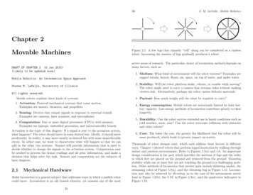
26S. M. LaValle: Mobile RoboticsChapter 2Movable Machinesactive areas of research. The particular choice of locomotion method depends onmany factors, such as:DRAFT OF CHAPTER 2 (8 Jan 2013)(likely to be updated soon)Mobile Robotics: An Information Space ApproachSteven M. LaValle, University of IllinoisAll rights reserved.Mobile robots combine three kinds of systems:1. Actuation: Powered mechanical systems that cause motion.Examples are motors, thrusters, and propellers.2. Sensing: Devices that output signals in response to external stimuli.Examples are cameras, laser scanners, and microphones.3. Computation: One or more digital processors (CPUs) with memory.Examples are laptops, embedded processors, and microcontroller boards.Actuation is the topic of this chapter: If a signal is sent to the actuation system,what happens? The robot should move in some desired way. Ideally, it should movepredictably. In reality, it may move mostly as desired but with some unpredictableerrors. In either case, we want to characterize what will happen so that we canadd in the other two systems. Sensors will provide information that is used todecide whether to change the signals to the actuation system. Computation maybe needed to process the sensor readings and all prior information, and make adecision that helps solve the task. Sensors and computation are the subjects oflater chapters.2.1Figure 2.1: A few legs that clumsily “roll” along can be considered as a rimlesswheel. Increasing the number of legs gradually produces a wheel.Mechanical HardwareRobot locomotion is a general subject that addresses ways in which a mobile robotcould move. Locomotion is an old branch robotics, yet remains one of the most251. Medium: What kind of environment will the robot traverse? Examples arerugged terrain, factory floors, air, space, on top of water, and under water.2. Stability: Will the robot platform shake, vibrate, or tumble while moving?The robot might need to carry a camera that streams video without makingviewers sick. Alternatively, perhaps the robot carries delicate materials.3. Payload: How much weight will the robot be required to carry?4. Energy consumption: Mobile robots are notoriously limited by their battery capacity. Low-energy methods of locomotion contribute greatly to theirlongevity.5. Durability: Can the robot survive extended use in harsh conditions such ascold weather, snow, rain? Can the robot overcome collisions with obstaclesand other robots?6. Cost: The lower the cost, the greater the likelihood that the robot will bemass produced, which leads to greater impact on society.Thousands of robot designs exist, which each address these factors in differentways. Chapter 1 showed robots that perform legged locomotion by walking throughindoor and outdoor environments. Refer to Figures 1.5(e) and 1.6. An importantdesign consideration is the gait, which specifies the motions of legs and the orderin which feet are placed on the ground and removed from the ground. Ensuringstability while one or more feet are not touching the ground is a challenging problem. Other methods of locomotion that involve gaits include slithering snakes, theswimming robot of Figure 1.9(a), and the vibrating bug in Figure 1.13. Locomotion may also be achieved by thrusting, as in the case of the autonomous motorboat in Figure 1.9(b), the UAV in Figure 1.9(c), and the quad-rotor helicopter inFigure 1.10.
2.1. MECHANICAL HARDWARE2728S. M. LaValle: Mobile RoboticsFigure 2.3: In 1985, the CMU URANUS mobile robot achieved omnidirectionalrolling by driving four Mecanum wheels, which were invented by Bengt Ilon.Figure 2.2: A low-cost robot built at the University of Illinois by extending theSERB open-source mobile design. The wheels and platform are cut from acrylicsheets. Each wheel is connected to a servo, and an Arduino microcontroller provides commands.Finally, the oldest and most common form of locomotion was offered by theinvention of the wheel. By comparing to the rimless wheel shown in Figure 2.1,rolling locomotion is the beautiful limiting case of having an infinite number oflegs that continuously move in unison. This case will be the main focus for theremainder of this chapter; however, keep in mind that mathematical models ofother locomotion methods have similar forms. Most of the robots from Section 1.1move by rolling.For rolling locomotion, each wheel is usually connected to an axle that is turnedby a motor. A simple, low-cost design is shown in Figure 2.2. At the high end,virtually any car, truck, or construction vehicle that has been designed for humanuse has been retrofitted for automated driving. An example is the Google car fromFigure 1.5(c). Large robotic vehicles at the high end use sophisticated electricaland mechanical systems that incorporate sensor feedback and gearing to deliverpredictable, reliable performance. Most of these build on extensive automotivetechnology that has been developed over the past century. In addition, many unusual rolling locomotion systems have been designed specifically for mobile robots.For example, the Mecanum (or Swedish) wheel (Figure 2.3) can roll both forwardas an ordinary wheel and perfectly sideways, which is quite unusual. This greatlyincreases the robot’s mobility, an issue which becomes important in this chapter.At the “unsophisticated” extreme, low-end robots can be constructed fromsimple components with a minimal amount of wiring and assembly skills. It isworthwhile to read popular, hobbyist robotics books (and build some robots!) tobecome familiar with widely available components []. Each wheel axle is normallyattached to the armature of a battery-powered, DC (direct current) motor. Stepper motors are a common choice because the 360-degree rotation cycle is divided(a) Lego NXT servo(b) Hobby servosFigure 2.4: Cheap, common servo motors: (a) A servo included in the Lego Mindstorm NXT robot kit. (b) A couple of servos that often appear on hobby vehicles,such as remote-controlled cars. (Source: Wikipedia)into a predetermined number of steps. This allows more accurate prediction ofthe amount of wheel rotation. The system should be well calibrated so that thenumber of steps can be reliably commanded and predicted. A precise clock signalcan be used to provide voltage pulses to the motor for prescribed time periods.Ultimately, performance is greatly improved by using a servo motor (or servo),which incorporates sensor feedback to ensure that the commanded amount of rotation has been achieved. Examples of commonly used servos are shown in Figure2.4. Servos can alter the steering direction of a robot in addition to driving itswheels.The remaining sections of this chapter describe the effects of commands thatare given to the mobile robot. A command is a digital signal that is convertedinto wheel actuation using a circuit such as the H-bridge shown in Figure 2.5(a).The battery is connected to the motor, but there are four controllable switches. Acheap solid-state device, shown in Figure 2.5(b), is used to convert digital signalsinto opened or closed switch configurations. Table 2.1 describes the response of
292.2. KINEMATICS OF PERFECT ROLLING ROBOTS(a)30(b)Figure 2.5: (a) An H-bridge circuit, which is a standard way to control a robotmotor. The power source and motor are represented inside of circles labeled “V”and “M”, respectively. There are four switches, S1 to S4 , that can be independentlyopen or closed. (b) A solid-state MOSFET device that implements the H-bridge.S110001S201011S301000S410010ResultActuate wheel in forward directionActuate wheel in reverseAllow the wheel to coastApply braking to stop the wheel quicklyShort circuit (useless)Table 2.1: The effects of five switch configurations from the H-bridge circuit fromFigure 2.5(a). A “0” indicates that the switch is open, and “1” indicates closed.The remaining nine possible configurations each produce one of these five results.the motor for several configurations of the switches.2.2S. M. LaValle: Mobile RoboticsKinematics of Perfect Rolling RobotsThe section describes the kinematics of rolling robots. The term kinematics meansthe geometry of motion without describing the forces that cause it. Every robot inthis section is modeled as a rigid platform that has attached wheels. Wheels areable to rotate, but some are driven by a motor and others just passively roll. Insome cases, the direction that the wheel is pointing may also rotate with respect tothe platform. If the direction is driven by a motor, then the robot can be steered.We want a precise account of where the robot will go when motors are turned onand the wheels are rolling. The robots are considered “perfect” in this section inthe sense that they behave in a predictable way that can be described with simpleequations. Section 2.4 covers the case in which they become less predictable dueto bumpy surfaces, slipping wheels, dying batteries, and so on.(a)(b)Figure 2.6: (a) The mobile robot moves in an infinite plane, with positions specifiedby x and y coordinates. (b) When the robot is placed at configuration (x, y, θ), itis moved from its home configuration (depicted by dashed lines) into the shownposition and orientation.2.2.1Single-Wheel DriveTo begin talking about the motion of a mobile robot, we will use the coordinatesystem shown in Figure 2.6(a). The robot moves along a “floor” that is the XY plane and extends infinitely in all directions. The position and orientation of therobot platform will be called the configuration. To uniquely describe every possibleconfiguration, we will use three parameters: x, y, and θ, which are written togetheras (x, y, θ). See Figure 2.6(b). The “home” configuration of the robot is (0, 0, 0).The special point is a location on the robot that has coordinates (0, 0) when therobot is at its home configuration. Any other configuration (x, y, θ) means thatthe special point on the robot is at position (x, y), and the robot is rotated by θwith respect to its home configuration. The x and y parameters may take any realvalue; however, to eliminate redundancy, θ is limited from 0 to 2π (including 0,but not 2π).Any point (xp , yp ) on the robot when it is in its home configuration will endup at(x xp cos θ yp sin θ, y xp sin θ yp cos θ)(2.1)if the robot is at configuration (x, y, θ). This is derived by first rotating the robotby θ and then translating (shifting) it by x in the X-direction and y in the Ydirection. Using a 2 2 rotation matrix, cos θ sin θ,(2.2)R(θ) sin θ cos θ
2.2. KINEMATICS OF PERFECT ROLLING ROBOTS31Figure 2.7: If wheels oriented in the directions shown, then is it possible for thisplatform to roll without any wheels skidding?the rotation part can be written as xxp cos θ yp sin θ R(θ) p .ypxp sin θ yp cos θ(2.3)32S. M. LaValle: Mobile Robotics(a)(b)(c)Figure 2.8: A top-down view of the wheels under a platform and their fixed directions: (a) If all wheel lines are parallel, then straight rolling occurs. (b) In thiscase, no instantaneous center of rotation (ICR) exists and the robot cannot roll.(c) The robot rolls with every wheel traversing a circle that is centered at the ICR.To perform the translation part, x is added to the first coordinate, and y to thesecond. This yields (2.1).Now consider attaching small wheels to the platform. Each wheel has a direction with respect to the X axis, when the robot is at configuration (0, 0, 0). SeeFigure 2.7. Here is a fundamental kinematics question:If some wheels are placed at specific positions and directions on theplatform, under what conditions is the platform capable of rolling?If the wheels are not aligned in a proper way, then some wheels may roll whileothers are skidding. How do we ensure that all wheels will roll?One of the easiest ways to ensure rolling is to point all wheels in the samedirection, as shown in Figure 2.8(a). Many other wheel placements will work,however, by considering an important concept from kinematics called the instantaneous center of rotation (ICR). Draw a line in the XY plane that is centered onthe wheel and is perpendicular to its direction. In other words, it is the axis aboutwhich the wheel rotates, but projected down into the XY plane. If all of the linesintersect at one point, then their common point of intersection is called the ICR.Our fundamental kinematics has a simple answer. The platform will roll ifand only if all lines are parallel or there is an ICR. Figure 2.8 shows examples.If the lines are parallel, then the robot will rotate along a straight line. If thereis an ICR, then the robot will rotate along a circular arc. The ICR is the centerof the circle that contains the arc. In the case of parallel lines, imagine that theICR is infinitely far away, in a direction perpendicular to the lines, and the robotmoves along a circle of “infinite radius”. All of our rolling robot models will beconstructed from the ICR principle.(a)(b)Figure 2.9: (a) A classic tricycle. (b) An old robot version: The Neptune robot atCarnegie Mellon University in 1984. Motors handle the “pedaling” and “steering”.
2.2. KINEMATICS OF PERFECT ROLLING ROBOTS3334S. M. LaValle: Mobile RoboticsFigure 2.11: If the front wheel is turned to φ π/2, then the ICR coincides withthe robot’s special point and the robot rotates in place.Figure 2.10: The important parameters of a tricycle.For a simple illustration, consider pedaling a tricycle (Figure 2.9(a)). Thefront wheel is powered by pedaling and is steered by turning the handlebars. Figure2.9(b) shows an old robotic equivalent of this. Figure 2.10 depicts the arrangementof wheels. The front wheel is shaded to indicate that it is powered. The whitewheels rotate passively and are always directed forward. If the front wheel ispointing straight ahead, then clearly the robot moves straight and forward. Iffront wheel is turned left, as shown in Figure 2.10, then it traverses a circle,centered at the ICR.We will now try to determine the configuration of the robot after it is driven.Suppose the robot starts at configuration (0, 0, 0) and the front wheel is steered tothe left by angle φ 0. See Figure 2.10. Let (xc , yc ) denote the coordinates of theICR. In this case, xc 0 and yc ℓ/ tan φ. To derive the position of yc , note thata right triangle is formed by the line through the special point and the front wheelcenter, and the two lines perpendicular to the wheels. The base of the triangleis ℓ and the height is yc . Its upper interior angle is φ; hence, from trigonometrytan φ ℓ/yc . The triangle height is also the radius rc of the circle traced out bythe robot special point as it rolls. The circle is centered at the ICR: (xc , yc ). Notethat as φ decreases to zero, rc yc increases to infinity. In the limiting case whenφ 0, the robot rolls straight, and the ICR does not exist (or is “at northerninfinity”).If the front wheel rolls distance dw along the circular arc, then what is theposition and orientation of the robot? Another way to express this is to say that thewheel has rolled ψ radians and has radius r. In this case, dw ψr, and we are backpto the original question. The center of the front wheel is distance rw ℓ2 rc2from the ICR. Hence, it moves along a circle of radius rw , centered at (xc , yc ).The back wheels, however, move along concentric circles of different radii becausethey are not distance rw from the ICR. To determine the robot configuration,we need to determine where the special point moves to and how much the robotrotates. Let ds denote the distance traveled along a circular arc by the specialpoint. The special point travels less than the front wheel because rc rw . Themoving robot is a rigid body that rotates counterclockwise about the ICR. Thedistance therefore scales according to the difference in radii: ds dw rc /rw . If thespecial point moves distance ds along the circle of radius rc , centered at (xc , yc ),then it rotates by angle θ ds /rc (this is just what fraction of the circumferencewas traversed, scaled by 2π). The position of the special point will be(x, y) (rc sin θ, yc rc cos θ)(2.4)The resulting configuration is (x, y, θ).If φ is negative, then the same method works, however, the robot will rotateclockwise, turning right the whole time. In this case, rc is negative and the circleradius is actually rc . Any angle φ can be handled except π/2 or π/2; seeFigure 2.11. In this case, the ICR coincides with the special point. The frontwheel traverses the circle of radius ℓ while the special point remains stationaryand the back wheels rotate around it. The rotation is counterclockwise and rc ℓin the case of φ π/2. It is clockwise and rc ℓ in the case of φ π/2. Notethat if φ π/2, it is equivalent to rolling backwards, which is not a problem.For example, φ 2π/3 is equivalent to φ π/3, but rotating the wheel in theopposite direction.Now consider the more complicated case in which the robot does not start fromits home configuration:1. The robot starts in some generic configuration (x, y, θ).
2.2. KINEMATICS OF PERFECT ROLLING ROBOTS(a)3536S. M. LaValle: Mobile Robotics(b)Figure 2.12: These two robot designs behave kinematically the same was thetricycle: (a) The rear wheels can instead be motorized; however, they must becoupled to roll together and have the same radius. (b) The pair of rear wheels canbe replaced by a single wheel to obtain a bicycle; however, side-to-side balancingbecomes an issue.Figure 2.13: The differential-drive robot has independent motors that power eachof the two rear wheels. A caster wheel is placed on the front for balance.2. The front wheel is pointing φ degrees from the forward direction.3. The front wheel drives distance dw along the arc.The task is to determine the resulting configuration, (x′ , y ′ , θ′ ). The first problemis that the ICR must be transformed. The ICR at (xc , yc ) (0, rc ) is rotatedby θ and then translated by x and y. Again, rc ℓ/ tan φ and may be positive,negative, or zero. The ICR when the robot is at configuration (x, y, θ) is then:(xc , yc ) (x rc sin θ, y rc cos θ).(2.5)Note that for (x, y, θ) (0, 0, 0), we obtain (2.4). The extension of driving alongthe circle from (2.4), is transformed to configuration (x, y, θ) to obtainx′ xc rc sin(θ θ)y ′ yc rc cos(θ θ)(2.6)θ′ θ θ.The model presented so far works for other wheel configurations. The rearwheels could be powered instead of the front wheel, as shown in Figure 2.12(a).In this case, careful motor coupling is needed to ensure that the wheels roll at theproper rate. If the robot is turning, then the inner wheel must rotate more slowlythan the outer wheel. This problem is solved in automobiles by the differentialmechanism. Figure 2.12 shows what happens if the two rear rears wheels arereduced to one: A bicycle is obtained. It rolls the same way as the tricycle,however, it must be capable of balancing. For a human-operated bicycle this isgreatly helped by conservation of angular momentum.2.2.2Differential DriveThe most popular kinematic model for mobile robots is the differential drive, whichavoids having to turn the wheels. Figure 2.13 depicts the wheel arrangement.(a)(b)Figure 2.14: Differential-drive robots: (a) The Roomba autonomous vacuumcleaner. (b) The Arduino Controlled Servo Robot (SERB) robot, which is a lowcost, open-source platform.
2.2. KINEMATICS OF PERFECT ROLLING ROBOTS3738S. M. LaValle: Mobile Robotics(a)Figure 2.15: The Segway uses a differential drive to send standing users on theirway. Rather than using an extra wheel for balance, a control system providesvertical stability.Figures 2.14 and 2.15 show some real examples. For a differential drive, two nonsteerable wheels are aligned so that a single perpendicular line crosses throughboth wheel centers. Both wheels have the same radius. Each wheel can be rotatedindependently. If they are rotated at different speeds, then the robot turns. Thereis usually a third wheel that simply keeps the robot from tipping over. A casterwheel is often used, as on the bottom of an office chair. The wheel orients itselfto roll in any direction that it is forced.Suppose that the two wheel motors are switched on so that each runs at aconstant speed. Let dl and dr denote the distance rolled by the left and rightwheels, respectively. The following simple motions arise:1. If dl dr 0, then the robot rolls straight and forward.2. If dl dr 0, then the robot rolls straight and backwards.3. If dr 0 and dl dr , then the robot rotates in place counterclockwise.4. If dr 0 and dl dr , then the robot rotates in place clockwise.For the last two cases, how far does the robot rotate? Also, what happens inall other cases, meaning that dl 6 dr ? These can be answered by determining(b)Figure 2.16: Car-like robots: (a) A car with a steered front axle. (b) A carwith Ackerman steering, which is allows the front wheels to turn in place whilemaintaining the existence of the ICR.the ICR and then applying the techniques from Section 2.2.1. It is clear that theICR will lie along the common perpendicular line through the rear wheels and thespecial point.All four of the simple motions above fit the following formula:rc ℓ(dl dr ).2(dr dl )(2.7)In the case of dr dl , then rc , which implies that the robot moves straight(along a “circle with infinite radius”). The formula in (2.7) correctly specifies rcfor all other values of dl and dr , assuming that each motor rotates at a constantspeed.2.2.3Car-Like RobotsAnother common variant of the tricycle is the car or car-like robot. In this casethere are two steered wheels in the front and two fixed wheels in the back. SeeFigure 2.16. The front wheels could be attached to a single steerable axle or theycould be rotate in place, which is like virtually all automobiles. If they rotatein place, then the steering must be coupled in a special way so that their perpendicular lines both intersect the ICR. This is referred to as Ackerman steering.If both front wheels are instead turned at the same angle, then skidding wouldoccur. As you may already know from automobiles, the power to the wheels could
2.3. DEFINING A CONTROL SYSTEM39be in the front, back, or both. This yields front-wheel drive, rear-wheel drive, andfour-wheel drive, respectively.The car moves in the same way as the tricycle. It is just a matter of figuringout the equivalent parameters. For the steered axle car in Figure 2.16(a), itsmotion is equivalent to having a single front wheel in the middle. The equationsfrom Section 2.2.1 correctly describe the motion using the same φ and substitutingℓ2 ℓ. Now consider the Ackerman steered car in Figure 2.16(b). If there werea wheel in front center and it is turned angle φ, then the car would turn withradius rc ℓ2 / tan φ. To achieve the same radius using the Ackerman steering,the steering angles shown in Figure 2.16(b) must satisfyrc ℓ1 /2 ℓ2 tan φ1(2.8)rc ℓ1 /2 ℓ2 tan φ2 .(2.9)andSolving for φ1 and φ2 yields the steering angles that avoid skidding.One important difference between the car-like robot and the other models hasbeen overlooked so far. In a car, there is usually a limit on how far the wheels canbe turned. Thus, if φmax is the limit, with φmax 0 and φmax π/2, then thesteering angle must be limited to φ φmax . This prevents the car from rotatingin place, which is a capability of the tricycle and the differential drive. Instead,the car has a minimum turning radius rmin ℓ2 / tan φmax , which corresponds tothe smallest circular arc that it can drive along.2.3Defining a Control SystemA control system is a convenient mathematical way to express the effects of commands on the states of a electrical or mechanical system that evolves over time.In the context of mobile robotics, the command usually indicates which motors toactivate, at what rate, for how long, and so on. This section merely describes theeffect of the command, without regard to how it is chosen. That is the topic ofcoming chapters.2.3.1Discrete-Time SystemsEvery control system has the following components:1. An command set U , which represents every command that can be given tothe system.12. A state space X, which characterizes every possible configuration or statusof the system. Examples are coming soon!1Common, alternative names for U are the input set or action set.40S. M. LaValle: Mobile Robotics3. A state transition equation, which specifies how the state changes under theinfluence of a command.In a continuous-time control system, the state transition equation is a differentialequation. In a discrete-time control system, it instead provides the next state as afunction of the current state and current command. Suppose x (which belongs toX) is the current state and u (which belongs to U) is a command that is appliedto the system. The discrete-time state transition equation isx′ fd (x, u),(2.10)in which the function f provides the next state x′ for every possible combinationof x in X and u in U. This idea appears in many other subjects, such as automatatheory, finite state machines, and planning algorithms.We now show take the kinematic models from Section 2.2 and make theminto control systems. Recall the tricycle from Figure 2.10. What are the possiblecommands? The power to the wheel motor and the desired steering angle arenatural candidates. To keep it simple at first, suppose that the motor is alwaysrolling forward at some constant rate. The command is the steering angle u φ.The command set is U [ π, π).Each state x is a configuration (x, y, θ) of the tricycle. The state space Xrepresents all possible (x, y, θ). For the first two coordinates, any (x, y) R2 ispossible. For θ, any value from 0 to 2π is possible; however, we must be careful todeclare θ 0 and θ 2π as the same orientation.We now have enough notation to specify the state and command, but whatdoes the “next state” mean? This means the state at some future point in time,usually when a special event occurs. In later chapters, this could correspond tothe arrival of a special sensor reading. For example, it might indicate that therobot has hit an obstacle. In this chapter, we define it to mean the state after apredetermined amount t 0 of time has passed.The state transition equation x′ fd (x, u) means that if the tricycle startsin configuration x (x, y, θ) and command u φ is applied, then it will be inconfiguration x′ (x′ , y ′ , θ′ ) after t seconds have elapsed. Assume that duringthe t time interval, the command cannot change. Figures 2.17 shows an example.Figure 2.18 shows the effect of the commands from Figure 2.17. Let x1 denotethe initial configuration. The first command u1 π/4 is applied for time t,and the robot traverses a semicircle to the left, arriving in state x2 fd (x1 , π/4).Recall that Equation (2.6) tells how to get x1 from x2 if the robot rotates by θr ,which in this case is θr π. At the next stage, u2 π/4 and the robot traversesa semicircle to its right, reaching x3 fd (x2 , π/4). After that, u3 0, the therobot moves straight to reach x4 . Finally, u4 is applied to yield the final state x5 .The discrete time model is conceptually simple. We apply a sequence of kcommands:(u1 , u2 , . . . , uk )(2.11)and the robot moves along k circular arcs or line segments. Some of its limitationsare:
2.3. DEFINING A CONTROL SYSTEM4142S. M. LaValle: Mobile RoboticsFigure 2.17: In our discrete-time model, the command is held constant over each t interval, and then it may switch to another command (or remain the same).1. It may be too restrictive to hold the command constant over each t. Therobot can move along a greater variety of curves if the command can varycontinuously over time. Section 2.3 allows this by using a differential equation to express the state transition equation.2. It is not physically feasible to instantaneously change the commands. Forexample, the wheel can not be changed from φ 0 to φ π/4 without goingthrough all angles in between. Alternatively, the motor can not be instantaneously switched on to a desired speed with going through intermediatespeeds. These problems are fixed by introducing more state variables, whichis the subject of Section 2.3.3.3. If we want to control the robot using the discrete-time model, then a clock orchronometer is needed to indicate precisely when t has elapsed so that thecommand is changed. We might instead want to change the command basedon some other event, which is sensed. This becomes crucial in later chapters,to develop robots that respond to their sensor readings, rather than simplya t timer expiring.2.3.2Kinematics as a Differential EquationConsider starting with a discrete-time model and making t very small. If somecommand u is applied, the robot will correspondingly move a small amount. Let x x′ x denote the small change in the state. For our robots of Section 2.2,we write x ( x, y, θ), meaning that x, y, and θ change by a small amount.Using the state transition equation (2.10),x x fd (x, u).(2.12)Figure 2.18: The special point on the robot traces out a path composed of circulararcs and line segments.We want to develop a way to obtain the state in the limit as t approaches zero.Note that xdx ,(2.13) tdtin which dx/dt is just the derivative with respect to time of every component ofthe state. For our robots, dx dy dθdx .(2.14)dtdt dt dtFor convenience, we will place a dot “.” over each variable to denote its timederivative. For example θ̇ means dθ/dt.For each value of x and u, we want to know the corresponding ẋ. This leadsto a differential equation known as the continuous-time state transition equation:ẋ f (x, u).(2.15)Once f is fully specified, the state velocity ẋ can always be determined. This canin turn be used to calculate future states via integration:Z tf (u(t), u(t)).(2.16)x(t) x0 0
2.3. DEFINING A CONTROL SYSTEM4344S. M. LaValle: Mobile R
Figure 2.3: In 1985, the CMU URANUS mobile robot achieved omnidirectional rolling by driving four Mecanum wheels, which were invented by Bengt Ilon. (a) Lego NXT servo (b) Hobby servos Figure 2.4: Cheap, common servo motors: (a) A servo included in the Lego Mind-storm NXT robot kit. (b) A couple of servos that often appear on hobby vehicles,