Transcription
Introduction to Polymer Physics.1Pankaj MehtaMarch 8, 2021In these notes, we will introduce the basic ideas of polymer physics –with an emphasis on scaling theories and perhaps some hints at RG.IntroductionPolymers are just long floppy organic molecules. They are the basicbuilding block of biological organisms and also have important industrial applications. They occur in many forms and are an intensefield of study, not only in physics but also in chemistry and chemicallectures. In these lectures, we will just touch on these ideas with anaim of understanding the basics of protein folding. A distinguishingfeature of polymers is that because they are long and floppy, thatentropic effects play a central role in the physics of polymers.A polymer molecule is a chain consisting of many elementaryunits called monomers. These monomers are attached to each otherby covalent bonds. Generally, there are N monomers in a polymer,with N 1. This means that polymers behave like thermodynamicobjects (see Figure 1). It will be helpful to understand some basicscales for the problem of polymers. First, entropic effects will be important and we will often askabout exerting forces on the polymers. For this reason it is helpfulto keep in mind that at room temperature 1pNnm 4.1k B T. To break covalent bonds between monomers, we need 1000K. Sothey are essentially never broken by thermal fluctuations However, “bending” and non-covalent interactions (electrostatics)compete with k B T. Monomers are typically of order 1 Angstrom or 1nm. Polymers are typically composed of N 10 109 monomers withlengths of 10nm 1m.It’s also helpful to look at some examples. Fig. 2 shows polymers ofvarious kinds that occur in biological systems.We see that there is a lot of diversity in polymers. What are thekey things we have to pay attention to. Well there are number ofthings that will be important. In particular, the things that we willcare about are:The references I have consulted arethe 2012 lectures of Polymer physicsfrom the 2012 Boulder Summer School.Notes and videos available here l-2012-lecture-notes.We have also used Chapter 1 of DeGennes book, Scaling concepts in PoylmerPhysics as well as Chapter 1 of M. DoiIntroduction to Polymer Physics, thisnice review on Flory theory https://arxiv.org/abs/1308.2414, as wellthese notes from Levitov available athttp://www.mit.edu/ levitov/8.334/notes/polymers notes.pdf.
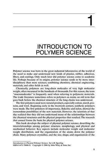
introduction to polymer physics.Polymer molecule is a chain: Polymeric from Greek polymer s having many parts;First Known Use: 1866(Merriam-Webster);Polymer molecule consistsof many elementary units,called monomers;Monomers – structuralunits connected by covalentbonds to form polymer;N number of monomers in apolymer, degree ofpolymerization;M N*mmonomer molecularmass.Examples: polyethylene (a), polysterene(b), polyvinyl chloride (c) and DNA The first important property is whether the polymer is a homopolymer – composed of a single kind of monomer – or a hetropolymer –composed of many kind of monomers. Most of the interesting biological polymers are hetropolymers (DNA with 4 bases, proteinswith 20 amino acids, etc.) The second major thing that will be important is how flexiblethe polymer is. The more flexible, the more entropic configurations that are available. All polymer bend but the question is howmuch? Another thing that will be important is if the polymer is charged.This is because electrostatic interaction compete with entropicinteractions. Finally, the basic topology is important. We can have a singlechain, or branching chains, or complicated topologies. We arefocusing almost entirely on single chains here.The final important thing about physics is that the properties ofpolymers are often strongly effected by the solvent in which they aredissolved. The reason for this is again because the solvent changesthe free energy of the polymers by changing the balance between entropic and energetic effects. In fact, we can characterize a polymer byits radius of gyration R defined the typical distance between the twoFigure 1: A polymer is composedof many monomers. Figure fromGrossberg Polymer lectures in BoulderSummer School 2012.2
introduction to polymer physics.3Figure 2: Polymers in living systems.Figure from Grossberg Polymer lecturesin Boulder Summer School 2012.Polymers in living natureDNARNAProteinsLipidsPolysaccharidesNUp to 101010 to 100020 to 10005 to 100giganticNicephysicsmodelsBioinformatics,elastic rod,charged funnels, ratchets,active brushesBilayers,liposomes,membranes? Someonehas to startUsesMoleculeends. In general, this is much smaller than a fully stretched polymersince polymers like to bend. In fact, we will see that typically thisradius goes like the number of polymers to some powerR Nν(1)The solvent, elasticity, and electrostatic interactions can change thispower dramatically from ν 1 for repulsive polymers to ν 1/3 inpoor solvents. This is summarized in Fig. 3.We can also directly measure this in experiment using X-ray crystallography in the small k limit.Neutral Flexible PolymersWe will start with “ideal” polymers. These are neural, flexible polymers that serve as an important starting point for understandingpolymer physics. Ideal polymers ignore all interactions betweenmonomers, except between neighboring monomers. Conceptually,they play the same role as an ideal gas for understanding the statistical mechanics of gases.
introduction to polymer physics.Polymer SizeMonomer size b 0.1nm; Number of monomers N 102-1010;Contour length L 10nm – 1m;Depending on how much polymer is bent,its overall size R varies widely and depends on solvent qualityLong-range repulsion Good solventR 1mR 100mm-solventR 10mmFigure 3: (Top) Polymer sizes in different solvents. (Bottom) Analogy tounderstand dramatic change in sizes.Figure from Grossberg Polymer lecturesin Boulder Summer School 2012.Poor solventR 100nmAstronomical Variations of Polymer SizeIncrease monomer size by a factor of 108: b 1cm; let N 1010.Poor solventGood solvent-solventLong-range repulsionFigure 4: In Freely-Jointed Chain, apolymer can be viewed as a randomwalk where monomers are connectedby bonds whose orientation is uncorrelated with the orientation of otherbonds. Notice that we have assumedthat there are no other interactions(electrostatic, excluded volume, etc).Picture from Wikipedia.Freely Jointed ChainWe can start by considering polymers as composed of monomersjoined by “bonds” between monomers. As a first approximation, weassume that the bonds are of a fixed length b but the orientation ofevery bond can vary and is uncorrelated with all other bonds (seeFigure 4). We will see that this very simplistic picture captures manyof the essential features of polymers— especially entropic effects.In fact, we will be mostly concerned with long polymers where thelength L is much larger than b so that the total number of monomersN L/b 1. In this case we expect entropy to dominate energeticeffects. The FJC model model does this by treating polymers as random walks. In this way, we can assign a probability to each allowedconfiguration. In doing this, we have neglected things like energeticinteractions and excluded volume.Let us now analyze the FJC in greater detail. Let us call the posi-4
introduction to polymer physics.tion of the j-th monomer r j . Let us also define the bond vector forthe j-th bond by τj r j r j 1(2)By definition, we know that the bond vectors satisfy the relationships τj b(3)h τj i 0(4)2h τi τj i b δij .(5)The first of these just fixes the length of the bond, the second that thebond is equally likely to be oriented in all directions, while the finalequation is simply the statement that the bonds are uncorrelated.Let us start with first calculating the mean end-to-end displacement of the polymer R. We know thath Ri h τj h τj i 0.j(6)jThis is simply the statement that polymer is equally likely to bepointed in all directions just like a random walk. However, we canalso look at the root-mean square displacement R defined byR2 h R · Ri h τj τk j,k h τj τk i b2 N.(7)j,kThis is the more accurate measure of the size of the polymer that wediscussed earlier. We see that this argument gives us a simple scalingrelationR bN 0.5 ,(8)and a scaling exponent ν 0.5 (defined in Eq. 1).At this point, it is worth better understanding what this exponentν means. Notice that if we haveR bN ν ,(9)then we can invert this relationship to getN 1R νb(10)This implies that the fraction of the polymer contained in a radius R0dfis just R1/ν R0 , where this equation defines the fractal dimension01d f ν . This is the usual way we define dimension since for d 1, 2, 3 we would expect number of things contained to go like R0 , R20 ,and R30 respectively. This is an interesting line of reasoning that tellsus something about the geometry of polymers.5
introduction to polymer physics.From FJC to Gaussian ChainIt will also be helpful to derive a general probability distribution forthis chain. To do so, we will make use of the general relationshipbetween random walks and the diffusion equation (Fokker-Planck)equation. It will be helpful now to consider a more concrete settingof a polymer in d-dimensions. Let us label the three components of τby τα with α 1, . . . , d labels the different directions. We known thath τ i hτα i 0.(11)αFrom symmetry, we conclude that in fact we must have that eachof these individual directions is zero. More tricky, is to consider thecorrelation functionhτiα τjβ i.(12)To calculate this, we rewriteh τi τi i b2 δij(13) hτiα τjα i b2 δij .(14)in component form to getαOnce again, by symmetry we know that all directions are equivalentso that we concludeb2hτiα τjα i δij(15)dFinally, since different components are uncorrelated, we can writehτiα τjβ i b2δ δd ij αβ(16)To proceed, we will write a recursive equation for the probabilityP( R, N ) that a polymer with N monomers has end-to-end displacement R. In particular, using Bayes theorem we can writeP( R, N ) Zd τ p( τ ) P( R τ , N 1),(17)where p( τ ) is just the probability of having an orientation τ for thelast bond. In the limit where N 1 and R b, we can perform aTaylor expansion of the right hand side. This yields (in componentnotation)P( R, N ) Z P( R, N ) P( R, N ) 1 2 P( R, N )d τ p( τ ) P( R, N ) τ τα τβ N2 αβ Rα R β R(18)!6
introduction to polymer physics.This yields using expectation values above the d-dimensional effective diffusion equation P( R, N )b2 2 P( R, N ) , N2d R2(19)with N playing the role of time and effective diffusion constantDe f f b2 /2d. We already know the solution to this equation is aGaussian distribution of the form d 2 2 dRd P( R, N ) (20)e 2Nb22πNb2In other words, the polymer behaves like a Gaussian chain. This suggests that we should be able to replace the more complicated FJC bya Gaussian model and still capture the long-distance physics of theproblem. In fact, the reason for this is that the chain is essentiallycomposed on N random steps each with variance b2 /d. Since variances of independent processes add, this tells us that We will returnto this universality in a little bit.This same argument also essentially tells us about the probabilitydistribution describing the difference between Rn Rm . In particular,we know that this will be a sum of n m terms each with varianceb2 /d. For this reason, we know that d d( Rn Rm )2 2 d2 n m b2 n , Rm ) P( Re(21)2π n m b2Polymers as springsBefore proceeding, this also gives us some idea about how entropicforces work. In the absence of external forces, polymers of courselike to contract. We can ask, how much force f is needed to fullyextend the polymer to distance R f . We will now treat this as a onedimensional problem in the direction of the force. In other otherwords, how much do you have to pull the polymer in order to . Wellwe know that we can also thing of this as a partition functionP( R, N ) e F ( R,N )kB T,(22)where F ( R, N ) is the effective free energy which we can identify asF ( R, N ) k B TR2.2Nb2(23)Notice this means that a polymer essentially behaves like a springwith effective spring constant that is proportional to the temperature:ke f f kB T,2Nb2(24)7
introduction to polymer physics.since partition function for spring is justPspring ( x ) e k e f f x2kB T(25)Now, we know if we exert a force f that the free-energy will be modified to yieldP( R, N ) e F ( R f ,N ) f R fkB T,(26)This combined free energy must be minimized at the force needed tostretch polymer implyingk B TR f F ( Re f f , N ) f RNb2(27)This basic idea that entropy can give rise to forces is an interestingone – and one that periodically gets revived in fundamental physicsas a possible origin of quantum gravity (most recently by Verlindehttps://en.wikipedia.org/wiki/Entropic gravity).Beyond Gaussian ChainsSo far we have ignored everything except for Gaussian effects. Howcan we incorporate these non-thermodynamic interactions. In general, this will be really hard. However, surprisingly mean-field theorydoes an incredibly good job of capturing the essential physics.Accounting for excluded volume/short range repulsive interactionsLet us start with the simplest version of mean-field theory. Let ustry to take into account excluded volume. In particular, let us writethe volume of one segment as vc . Then the probability that a givenmonomers does not overlap a second monomer is just 1 minus thefraction of volume occupied by the second segment in d-dimensionsis justq (1 vc /Rd ).(28)In general, for a polymer composed on N monomers, there are N 2such potential overlaps. The probability that none of the segmentsoverlap is given by2w( R) q( N ( N 1)/2) (1 vc /Rd ) N R3 vc e N 2 vcRd(29)where in writing this, like in all mean-field models we have ignoredthe correlations between monomers.Now we make the further assumption, that the we can write theprobability of having a polymer of length R with excluded volume8
introduction to polymer physics.interactions, p f lory ( R) is just the probability of having a Gaussianchain of length R given by Eq. 20 times the probability that nomonomers occupy the same volumep f lory ( R) p( R)w( R) d R22Nb2 e e2 N dvcR e N 2 vcRd 2 dR 22Nb(30)(31)This allows us to identify an effective scaling free energyF d R2N 2 vc .d2Nb2R(32)The equilibrium R will minimize this energy. Let us now differentiate this equation to get dN 2 vcRd 1 dR 0Nb2(33)which yields the scaling relation3R N ν N d 2 .(34)Thus, we see that the repulsive interaction have modified our exponent ν from the ideal model where ν 1/2 to ν 3/5 in d 3dimensions and ν 3/4 in two dimensions. Surprisingly, this is ingood agreement with experiments!Basic Phase Diagram of PolymersWe thus far considered only repulsive interactions. One can alsothink about attractive interactions. Obviously, attractive interactions will make the polymer more compact. With attractive interactions and hard core repulsion due to steric occlusion, the polymermonomer would like to stay as close as possible. In particular, weexpect the density of monomer to be O(1). Thus, we expect thatN/Rd 1, so that we haveR N 1/d .(35)These basic considerations allow us to think of a stylized phasediagram for polymers. Since the temperature controls the relativeeffects of entropic versus energetics. Thus, at low temperatures wewould expect that attractive interactions dominate and the polymeris “collapsed” with R N 1/d . At some transition temperature oftencalled T Tθ , we expect a phase transition to an extended phase9
introduction to polymer physics.10where R N v . These two regions are separated by a critical regionsaround T Tθ where R N 1/2 . This is summarized in Figure 5.7We will not have time to work through this in detail. However, rest2. Collapseassured this can be made more precise using field theoretic methodsThe case of attractive interaction may also be mentioned here. With attraction, and hard-core repulsion, themonomers wouldfromlike to stayas closeTheseas possible. areThis givesa more interestingor less compact packingandof spheresso that theand methodsRG.quiteinvolvedmonomer density inside a sphere enclosing the polymer is O(1) in N . Note that the density for the repulsive caseN/R N 0, for large N . A compact phase, also called a globule, would then havecalculations.1d1 dνR N 1/d , i.e., ν d.(compact)(2.13)The collapsed state is not a unique state and the polymeric nature is important in determining its overall property.One expects a generic phase diagram, as schematically depicted in Fig.2, with a theta point at T Tθ , a hightemperature (T Tθ ) swollen or coiled phase and a low temperature (T Tθ ) compact phase. This will be discussedin detail in Section V.Figure 5: Phase diagram of polymersfrom "Flory Theory of Polymers"(arxiv:1308:2414).1/2R N1/dνR NR NT TθT TθT TθIdealCollapsedExtendedFIG. 2: Schematic phase diagram of an isolated homopolymer. At high temperature T Tθ , the polymer is in a swollen phase(right), whereas one expects a compact globule at sufficiently low temperatures T Tθ (left). These two regimes are separatedby a transition regime at T Tθ (center) where the polymer behaves more or less as a Gaussian chain, at least in d 3.III.THE EDWARDS CONTINUUM MODELA.Discrete Gaussian modelThe central limit theorem, as explained in Appendix A, allows us to describe a polymer by the distributionW (r0 , . . . , rN ) of N bonds, τ1 r1 r0 ,. . ., τN rN rN 1 , each having a Gaussian distribution, as"#&'% d/2NN!!11 τj2p (τj ) W (r0 , . . . , rN ) ,(3.1a)exp 222πb2bj 1j 1Understanding Universalityand Self-Similarity: From(3.1b)WLC back Z exp [ βH ],wherewehaveintroducedtheGaussianHamiltonianto FJC 1GβHG GNN1 (1 ( 2τ 2(rj rj 1 )2 ,2b2 j 1 j2b j 1(3.1c)One ofwiththemostpowerfulinteresting ideas to come out of polythe partitionfunctionZ (2πb ) and.The Gaussian Hamiltonian is another representation of a polymer where the monomers are connected by harmonic2 . Thesesprings (Fig. 1c).any nonzerothe equipartitiontheorem gives τ %/b have d, whichtheirallows theoriginbondsmer physicsis Attheideatemperature,of scalingideasinto have a nonzero rms length. The size of the polymer is given by R % db N .the work of Michael Fisher and collaborators on phase transitions,but polymers are arguably the place where they were most widelyand successfully used outside this original setting. The basic ideaof the scaling theory is that at long distances, the physics should beindependent of the scale at which I view the problem at short distances.G2 N d/2222j2One of the defining properties of random walks is that they areself-similar. This essentially means that as I view a random walkat different scales, it essentially looks the same 3 . The under lyingreason for this is that we we ask how the radius of the random walkscales with the number of steps, this takes the form of a powerlaw:R Nν.(36)To see why power laws are special, let us consider two kinds offunctionsAf l (x) α(37)xHere we will follow the discussionof Doi as wall as Bhattacharjee et al inarxiv:1308:24142A great demonstration of this canbe found from Wolfram applet arityInRandomWalk/
introduction to polymer physics.and xBe ξf s (x) .(38)xαNotice that the second of these has a natural length scale associatedwith it ξ whereas there is no length scale with the first function.Imagine now, we measured x on a different length scale x 0 λx,the we we that by setting A0 Aλ α the functional form of f l ( x )remains invariant. Thus, no matter the scale λ at which one looksthe basic power law behavior remains the same. This is the idea ofscale invariance. We can contrast this with the function f s . If λx ξwe cannot simply rescale the parameter B and then obtain the samefunctional form.In fact, one can go a little further. We have shown that any powerlaw function is scale invariant. In fact, one can also show the oppositemust also hold: a scale invariant function (defined below) must takethe form a power law. Assume we have a scale-invariant function sothat:f (λx ) λ p f ( x )(39)for all choices of λ (this is known as continuous scale invariance). In thiscase, we see that by setting λ 1/x, we get thatf (1/x ) f (1) x p .(40)Substituting, y 1/x we come to the conclusionf (y) y p .(41)Thus, we see that continuous scale invariance implies power lawscalings and vice versa.In the context of polymers, let us revisit the FJC model, and inparticular Fig. 4. Notice that the scale b0 we chose for the length ofthe links and the number of corresponding monomers N L/bwas somewhat arbitrary. We could have just as easily chosen a different scale b0 and different number of monomers N 0 . However, weexpect that the long distance physics should be independent of thesechoices. In particular, for long polymers L 1, we expect the physicsto be independent of all these choices.Consider the probability P( R, L) that a polymer of length L hasend to end displacement R. In principle, this probability depends onall the exact details of our microscopic model. However, we knowthat for long distances this should only depend on L. Let us nowimagine changing the macroscopic scale of the problem so thatL λL,(42)11
introduction to polymer physics.while keeping the microscopic scale b fixed. This is called a scaletransformation. Notice in Flory theory, we will be keeping the microscopic scale fixed. In particular, since we haveR b1 ν ( Nb)ν Lν(43)Thus, under a scale transformation L λL and R λν R. Theprobability will show scaling ifP( R, L) λ x P(λν R, λL),(44)for all λ. Let us now choose a λ 1/L. This yields R R11P( R, L) x P( v , 1) x P ( v ),LLLL(45)where in the last line we have defined the scaling function P .Now, we know thatZdr d P( R, L) 1.(46)This implies thatZ R1P( x )xLLZ RL x dr d P ( x )L1 dr dSubstituting r r̃Lv givesL x LdνZdr̃ d P ( R̃)(47)This implies that x dν and our scaling function takes the form R1P()LvLdν(48)We can compare this with our expression in Eq. 20 using L Nband ν 1/2. In particular, we have thatP( R, L) d2πLb d2e d R22bL (49)and indeed this scales as L dv .More scaling analysis of polymers in solutionsThus far we have basically considered an isolated polymer. However,polymers often occurs in solution. We are interested in understanding polymers in a solution. After all the cell, is a very crowded placeas this famous picture from David Goodsell shows (see Fig. ?. Wewill largely confine ourselves to some simple scaling arguments.12
introduction to polymer physics.13Figure 6: This illustration shows across-section of a small portion of anEscherichia coli cell. The cell wall, withtwo concentric membranes studdedwith transmembrane proteins, is shownin green. A large flagellar motor crossesthe entire wall, turning the flagellumthat extends upwards from the surface.The cytoplasmic area is colored blueand purple. The large purple moleculesare ribosomes and the small, L-shapedmaroon molecules are tRNA, and thewhite strands are mRNA. Enzymes areshown in blue. The nucleoid regionis shown in yellow and orange, withthe long DNA circle shown in yellow,wrapped around HU protein (bacterialnucleosomes). In the center of thenucleoid region shown here, you mightfind a replication fork, with DNApolymerase (in red-orange) replicatingnew DNA. copyrigh David S. Goodsell1999.Critical ConcentrationsConsider polymers in solution at some concentration c of monomersin solution. We know that if this concentration is very small, we canthink about the polymers as isolated and non-interacting. However,at large concentrations where the distance between polymers approaches the radius of the polymers themselves R g , the properties ofthe polymer solution will differ from the isolated polymers. This isdepicted in Fig. ? from Doi’s book.Let us denote the concentration that separates these regimes byc . We can actually recover this from simple scaling arguments. Weknow thatc N/R3g(50)However, we know that R g N ν so that we havec N 1 3ν(51)Recalling that ν 3/(d 2), we see that for d 3 that we have thatc N 0.8 so that if N is very large that there is strong interactionseven at very small concentrations. For example, polyesterene withmolecular weight 106 starts to interact at 0.5% weight concentrations.Correlations length of polymersSince the polymers are interacting in solution, the polymer solutionis no longer scale free but instead defined by a correlation length ξ.Let us now try to use dimensional analysis and scaling arguments totry to figure out the scaling properties of the correlation length. By
introduction to polymer physics.14Figure 7: Figure 2.1 from Doi showingmeaning of critical concentration.dimensional analysis, we know that we we expect that the propertiesof the polymer will take the formξ R g f (cb3 , N ),(52)where f is some arbitrary function of the dimensionless numbers cb3and N.We will ask what happens as we “coarse-grain” the chain so thatwe group together some segments into a smaller number of segments: N λ 1 N where λ 1. In particular, we expect that forlarge N the fundamental physics should not change under such acoarse graining. Under such a transformation, we have that the concentration will decrease like N but the length scales will scale as λν :N λ 1 N, b λν b, c λ 1 c(53)Since the correlation lengths and the radius of gyrations are physicalquantities, they must be invariant under such a transformation so thatξ R g f (λ3ν 1 cb3 , λ 1 N )(54)
introduction to polymer physics.Let us choose λ N, to get thatcb3, 1)N 1 3ν 1 3ν 1N3 R g f (cb, 1)b3c R g f ( , 1)c c Rg F ( )c ξ Rg f ((55)This shows us the correlation function is a scaling function of c/c .To proceed, we will make some more scaling assumptions. Inparticular, for c c , we know the correlations do not depend of thedetails of the polymer involved. In fact, the correlation length mustbe independent of N. Since we know that the powers of N come fromR g N ν and c N 1 3ν . This means thatF(c) c cc x N x(1 3ν) .(56)This implies that since ξ is independent of N thatx ν/(1 3ν)so that we getξ Rg cc ν/(1 3ν)(57),(58)which for d 3 implies ξ c 3/4 which has been confirmed experimentally.15
A polymer molecule is a chain consisting of many elementary units called monomers. These monomers are attached to each other by covalent bonds. Generally, there are N monomers in a polymer, with N 1. This means that polymers behave like thermodynamic objects (see Figure 1). It will be helpful to understand some basic