Transcription
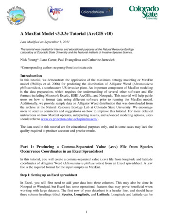
A MaxEnt Model v3.3.3e Tutorial (ArcGIS v10)Last Modified on September 1, 2011This tutorial was created for internal and educational purposes at the Natural Resource EcologyLaboratory at Colorado State University and the National Institute of Invasive Species Science.Nick Young*, Lane Carter, Paul Evangelista and Catherine Jarnevich*Corresponding author: neyoung@nrel.colostate.eduIntroductionIn this tutorial, we demonstrate the application of the maximum entropy modeling or MaxEntmodel (Phillips et al. 2006) for predicting the distribution of Alligator Weed (Alternantheraphiloxeroides), a southeastern US invasive plant. An important component of MaxEnt modelingis the data preparation, which requires the understanding of several other software and fileformats including Microsoft Excel , ESRI ArcGIS , and Notepad . This tutorial will help guideusers on how to format data using different software prior to running the MaxEnt model.Additionally, we provide sample data on Alligator Weed distribution that was downloaded fromthe archive at the Natural Resource Ecology Lab at Colorado State University. We encourageusers to send us comments and suggestions on how to improve this tutorial. For more detailedinstructions on how MaxEnt operates, interpreting results, and advanced modeling options, usersshould refer to www.cs.princeton.edu/ schapire/maxent/ .The data used in this tutorial are for educational purposes only, and in some cases may lack thequality required to produce accurate and precise results.Part 1: Producing a Comma-Separated Value (.csv) File from SpeciesOccurrence Coordinates in an Excel SpreadsheetIn this tutorial, you will create a comma-separated value (.csv) file from longitude and latitudecoordinates of Alligator Weed (Alternanthera philoxeroides) from an Excel spreadsheet. A .csvfile is the required format for the input samples in MaxEnt.Step 1: Setting up an Excel spreadsheetIn Excel, you will first need to add your data into three columns. This may also be done inNotepad or Wordpad, but Excel has some operational features that may prove beneficial whenworking with large datasets. The first row of your datasheet is a header line, and should havethree column headings titled: Species, Longitude, and Latitude. Longitude and latitude can be1
substituted with Easting/Northing, X/Y, etc. Under these headings, your data should be enteredor copied. If your data is in a shapefile format, Excel is able to open .dbf formatted data.IMPORTANT! Before you continue, make sure the coordinates you are using are in longitudeand latitude for this example! MaxEnt can handle most coordinate systems provided that the .csvfile coordinates match the coordinate system of the spatial data layers.When you have completed the data compilation, save the file in your working folder (e.g. all ofthe steps following will save documents under the Alligator Weed working folder).Step 2: Converting your Excel file to a csv fileOnce your data in the Excel fileare ready, you will need toconvert and save it in yourworking folder as a .csv file. Inour case, the original file islabeled Alligator Weed.xlsTo convert this file to a csv fileclick File then Save As. Awindow will appear. Save the filein the Alligator Weed folder andunder Save as Type, choose CSV2
(Comma delimitated) (*.csv). Then click Save.Now you have created a .csv file that is ready to be used with MaxEnt. The new file should be inyour Alligator Weed folder. You can check to see if the conversion worked by making sure thatthere is a .csv at the end of the file name.Well done! You have created a comma separated value (.csv) file from coordinates in an excelspread sheet!Part 2: Modifying Environmental Layers to be the Same Extent (geographicbounds and cell size) Using ArcGISBackground:This part of the tutorial walks you through the steps required to modify environmental layers inArcMap so that all your spatial data (i.e. independent or predictor variables) have the sameextent (same geographic bounds and cell size). MaxEnt requires all the environmental layers bein raster format and have the exact same cell size, extent and projection system (e.g., geographicor UTM) in order to execute a model.Step 1: Loading layers into ArcMap and opening the Extract by Mask toolBefore you start modifying layers, make sure you have adequate space to work with large files.You will need at least 6 giga bytes (GB) of free space to complete these modifications. Also, youmay want to create a new folder to store and separate the modified layers. Create this folder inthe Alligator Weed folder and call it ModLayers.Open a new map in ArcMap. Click on the add data iconand navigate to the location ofyour environmental variables. In this example they are within a folder called BioRasters. Add allthe environmental layers to the map. In our example, this will be the bio 1, bio 2, bio 3 etc.(The environmental layers are coded to correspond with thelist of variables at the end of this tutorial) ArcMap may popup a window that says if you would like to create pyramids,click Yes. This will help display the raster layers quickly, butit might take a while for ArcMap to load the raster layers.First, you will need to turn on the spatial analyst toolset.Click on Customize at the top of your ArcMap screen, andscroll to Extensions. An extensions window will appear.Check the Spatial Analyst box and click Close.3
Click on the Toolbox iconand from the list of tools extend theSpatial Analyst tool. Under Extraction select Extract by Mask.Step 2: Setting up Extract by Mask and the extent and cell size in spatial analystIf your environmental layers happen to be larger than the area you are interested in modeling,this step allows you to clip them down to your area of interest and set all layers to have the sameextent, cell size, and coordinate system (a requirement of MaxEnt). This step can also be used toset your extent, cell size and coordinate system if your environmental layers are already clipped.A window should appear that looks like the one below for the Extract by Mask tool (locationdescribed above).For the Input raster click on the folder iconand browse to the BioRasters folder andselect the bio 1 variable.For the Input raster or feature mask datafield, use theicon to browse to a raster orpolygon that represents the spatial boundaryyou intend to model.Note: For this Alligator Weed example, thespecies is known to be most prominent in thesoutheastern states, therefore the mask is ashapefile named SE states.shp that wasalready created.4
Save the Output raster as bio 1 under the folder ModLayers you created previously. This iswhere all the modified layers you create from this step will be saved.In order to set the coordinate system, cell sizeand extent, click on the Environments button in the bottom right of the window*.Extend the variables Output Coordinates,Processing Extent, and Raster Analysis.*Note: If this is the first environmental layerthat you want to clip, you do not need to setthe Environments The first clipped layeryou create will become the layer you use todefine your environments for all otherenvironmental layers in the model (in thisexample we first used the boundary layer tomask bio 1 which will then be used in theenvironmentsfortheremainingenvironmental layers [bio 2-bio 19]). It maybe a good idea to use the Environments forthe first environmental layer if it is notalready in your intended coordinate system.The window to the right is displayed:Use theicon to set theCoordinates variable to bio 1BioRasters folder. The namecoordinate system will appear in thebelow the input field.Outputin theof thewindowFor the Processing Extent and Snap Raster variables, browse to a raster you know that alreadyhas the extent you wish to match. In this case it is bio 1 as well.For the field of Cell Size under the Raster Analysis variable, you will want to enter yourenvironmental layer that has the smallest cell. In this case we will choose the same layer theother variables: bio 1. The true cell size value will appear in the window below the input field. Itwill reflect the units from which your coordinate system is based.Click OK.5
By the end the windows should look something like this:Now Click OK.Repeat this process until all of your environmentalrasters are extracted to the extent and contain thecell size and coordinate system you intend.IMPORTANT! Within the Environments, youmust use one consistent layer to set the coordinatesystem, extent, and cell size to ensure all areexactly the same. Here the layer bio 1 is used forall environmental layers to match.Congratulations! You have modified all your environmental layers to be the same cell size andextent. This can be the most time consuming part of the data preparation.Part 3: Converting Environmental Rasters to ASCII FormatThis section demonstrates how to convert environmental raster layers to ASCII format. Allenvironmental layers must be in ASCII format to run MaxEnt.Step 1: Loading raster layers into ArcMap and opening the Raster to ASCII tool.Before you start, create aASCII Environmental layers.newfolder6intheAlligator Weedfolderlabeled
Open ArcMap and select a New Empty Map.Click OK.Click on the add data iconand navigate to theAlligator Weed folder, then to the ModLayersfolder and select one of the environmental rasters thathas already been modified to be the same extent andcell size as the other layers (i.e. bio 1).Click Add.Open the Toolbox window by clicking on the toolbox icon.In the Toolbox window double click Conversion Tools then FromRaster, and then double click on the Raster to ASCII tool.Step 2: Converting raster layers to ASCII files.For the Input Raster click on the folder iconthe bio 1 file in the BioRasters folder.and navigate toFor the output ASCII raster file, click on the folder iconandnavigate to the new folder you created in the Alligator Weed folderlabeled ASCII Environmental layers. Save the ASCII layer as thesame name as the original layer name bio 1.IMPORTANT! Make sure the File (*.ASC) is selected in Save astype.Click Save.7
The Raster to ASCII window should look like this:You may need to manually change the file name to .asc instead of .txt or .asc.txt. If the file is notis .asc format, MaxEnt will not be able to read it.Click OK.A progress scroll will appear as it runs the conversion. This can take a while.Now you should have a file called bio 1.asc in the ASCII Environmental layers folder.Repeat the above steps for the remaining raster layers that need to be converted to ASCII for theMaxEnt model.Congratulations! Now you have created ASCII files from your environmental layers that you canenter into MaxEnt.Part 4: Running the MaxEnt ModelIn this part of the tutorial, you will learn how to download and run a MaxEnt model. This tutorialwill also explain where to find MaxEnt on the web and how to download the module. MaxEnt, amachine learning program (Phillips et al. 2006), is a powerful tool used to predict species’ spatialdistribution (current and potential) using presence point locations and environmental layers. Thistutorial covers the minimum information needed to run the MaxEnt model. Additional ntwebsite(www.cs.princeton.edu/ schapire/maxent/).8
Step 1: Downloading MaxEntTo begin, go to the website http://www.cs.princeton.edu/ schapire/maxent/ to download theMaxEnt software. On this page, you will find links to two papers that may help inform you moreon mathematical and theoretical aspects of how the MaxEnt algorithms work. Further down thepage under Terms of Use, you will see where to enter your Name, Institution, and Email address.Fill in the requested information, and select version 3.3.3e (or latest available version).When you are finished, click the Accept terms and download button.A new page should come up that explains how todownload the software. You can download each of theMaxEnt’s three files separately (i.e. maxent.jar,maxent.bat, readme.txt) or you can download all of themin .zip file.Save the .zip folder to whatever workspace you areworking off of.Once your download is completed, you should see the three MaxEnt files in your folder.To open the MaxEnt model, go to this folder and click on the maxent.bat file.Step 2: Defining MaxEnt Background SelectionThis section describes how to define how MaxEnt selects background samples (also calledpseudo absences) or how to provide MaxEnt with absences. These samples will be used toestimate the environmental layers across the entire extent or landscape used to model the speciesdistribution. The background samples used when developing a distribution model can havesignificant impacts on the model results (for more information on this topic see Elith et al. 2011).Often we are modeling species within the United States. One method used to limit where thebackground points are selected from is to only let MaxEnt select from counties where you havesample locations. This limits the background point to areas that we assume were surveyed for thespecies which provides MaxEnt with a background file with the same bias as the presencelocations.Often, we may be modeling a species distribution in another country or at small extent where theuse of counties to select background points from does not make sense. In these cases, it may bebetter to use the minimum convex polygon to define the area where MaxEnt will draw itsbackground samples from. For the purpose of this tutorial, we will not describe in detail how todo this, but it important to be aware of this technique.9
Another method to select background samples is to provide your own background points toMaxEnt. This serves two purposes: (1) you select the specific background locations MaxEnt usesto develop the model and (2) this will speed up the MaxEnt model process. Deciding whatbackground samples to include in the model can be difficult. The best suggestion is to usepresence points for another species that was part of the same survey as the focus species.Which method you use for background samples for MaxEnt depends on the data available, thegeographic characteristics of the area, and the size of the extent you are modeling.For this example, we will select background points from the counties where we have presencedata for alligator weed. To accomplish this, you will have to clip all the environmental layers youuse for the model (see Part 2, step 2 for details) to the counties that have alligator weed presencelocations. You will then use the clipped environmental layers to develop the model and projectthe model (more on this in step 3) to the extent you wish to model the distribution of AlligatorWeed. The steps to create the clipped environmental layers are outlined below:First, open ArcMap10 and load your Alligator Weed.csv file of the locations points and make ita shapefile by right-clicking on the layer selecting Data then select Export Data. Save theshapefile in the Alligator Weed folder and name it Alligator Weed.shp. Make sure to add thenew layer to the map. Now add the US counties GCS wgs84.shp to the map located inAlligator Weed.10
We are now going to select only thecounties that have a recorded presencewithin them. To do this, go to Selectionin the top menu bar then Selection ByLocation In the Select By Location window, select US counties GCS wgs84 as the Target layer, makeAlligator Weed the Source layer, and choose Target layer(s) features intersect the Sourcelayer feature as the Spatial selection method. Leave the apply search distance unchecked.Click Apply. Then click OK.11
The counties with presence points should be highlighted. To create a new layer with thesecounties right click the US counties GCS wgs84 layer in the table of contents and selectSelection and then Create Layer From Selected features.A new layer should appear in the table of contents called US counties GCS wgs84 selection.Now we will convert the new layer to be a raster. To do this go to ArcToolbox then ConversionTools then To Raster and select the tool Polygon to Raster. Select US counties GCS wgs84selection for the Input features, save the file in Alligator Weed as bias file and set the cell sizeto be the same as the bio 1 grid file in the BioRasters folder. Leave the other fields blank andclick on the Environments button.In the Environments window, set theExtent, Snap Raster, Cell Size, andMask all to be the bio 1 grid in theBioRasters folder. Click OK.12
A new raster should appear that only covers the counties selected. We will want to convert thenew raster to have a value of 1 in all selected counties and a value of “NoData” everywhere else.To do thism, go to ArcToolbox then to Spatial Analyst Tools then Map Algebra and selectRaster Calculator. Enter the following Con statement into the window and save the file underAlligator Weed as bias filecon:Con Statement: Con (“bias file” 0, 1, “bias file”)13
This will create a new layer in the table of contents. We will need to convert this layer to be anASCII file. To do this go to ArcToolbox then Conversion Tools then to From Raster thenselect Raster to ASCII. Make sure to set the Extent, Snap Raster, Cell Size, and Mask all tobe the bio 1 ASCII file in ModLayers that you created earlier. Save the output file asbias file asc. You will include this file in the Bias window in MaxEnt settings (see Bias in step4).Step 3: Opening MaxEnt and Setting Up a RunBefore starting MaxEnt, navigate to the Alligator Weed folder and create a new folder labeledOutputs. This will be the folder where the outputs created by MaxEnt will be stored.IMPORTANT! When environmental layers are very large, you may get an “out of memory”error when you run the program. The best way to fix this problem is to give MaxEnt access tomore memory. To do this, you will edit the maxent.bat file and increase the memory from 512 to1024 (or multiples of 512 such as 512x2, 512x3, 512x4 depending on your computer’s RAM).Memory size of 512 indicates the 512mb of your computer’s total RAM will be allocated forrunning MaxEnt model.To do this, first right click on the maxent.bat file in your working folder and select Edit.A Notepad window shouldappear like the one shown onthe right.14
You can change the amount ofmemory that MaxEnt uses bysimply changing 512 to 1024.This is how the window shouldlook.Once you have changed the memory, click File and Save and close the window.To open MaxEnt, click on the maxent.bat file. A window should open that looks like this:To begin, you must providea Samples file. This file isthe presence localities in.csv format (see Part 1). Forthis demonstration, we willuseAlligator Weed.csvwithin the Alligator Weedfolder. Navigate to this fileby clicking the Browsebutton under Samples, oryou can type in the filepath.Next you have to providethe Environmental Layersused for the model. Thiswill be the folder that contains all your environmental layers in ASCII format (they must have an.asc file extension) with the same geographic bounds, cell size, and projection system. In ourcase, the folder containing our layers is found in the ASCII Environmental layers folder.Navigate to this folder by clicking the Browse button under Environmental Layers, or type inthe file path. Notice how you can change the environmental layers to either continuous orcategorical. If any of the layers you include in your environmental layers are categorical (e.g.vegetation type), make sure you change them by clicking on the down arrow and choosingcategorical.An Output folder also needs to be selected. This will be the folder where all the MaxEnt outputswill be stored. For this exercise, we will use the folder created earlier named Outputs. Navigateto this folder by clicking the Browse located next to the Output Directory, or type in the filepath.15
You can leave the Projection Layers Folder/File window blank if you do not intend onproducing future scenarios. For the Alligator Weed we will input one projected model for 2020.Assuming these projected climate variables arealready available, navigate to them by clicking onthe Browse located next to Projection LayersFolder/File.Depending on where your projected climatevariables are located, the browse window willlook similar to this:To add a second or third projection, one cannotnavigate using Browse. Instead, place a comma atthe end of the first file path, enter a space, thentype in the second path name (if your projectedvariables are within the same folder simply copyand paste the first path name but be sure to change the last file name from 2020 to your newprojection file name).Make sure that the Create Response Curves, Make Pictures of Predictions, and Do jackknifeto Measure Variable Importance boxes are all checked.Keep the Auto Features box checked and leave the Output Format as Logistic and the Outputfile type as .ascNow, the MaxEnt GUI (graphic user interface) should look like this:16
Step 4: MaxEnt SettingsReplicates (Number of Runs)MaxEnt allows the ability to run a model multiple times and then conveniently averaging theresults from all models created. Using this feature in combination with withholding a certainportion of the data for testing (see Random Test Percentage below) enables the ability to test themodel performance while taking advantage of all available data without having an independentdataset. Executing multiple runs also provides a way to measure the amount of variability in themodel. To set the replicates in MaxEnt, go to Settings and then enter the number of run in theReplicates field. In this example we will use 15.Reducing disk space and increasing speed (optional setting)When the only output needed from a MaxEnt run is the averaged results from multiple runs(replications), you can change the model setting to turn off the “write output grids.” This willprevent MaxEnt from writing output grids from individual runs and only output the summarystatistic grids (e.g. Average, Minimum, Maximum, etc.) from all the runs. This will speed up the17
total run time and decrease disk space. You can turn off the “write output grids” option bygoing to Settings, selecting the Advanced tab and then de-check write output grids.Random Test Percentage (Test data)One way to evaluate model performance is to use the Random test percentage setting in MaxEnt.This setting allows you to withhold a certain percentage of your presence data to be used toevaluate the model’s performance. This is important because without these test data, the modelwill employ data used to develop the model (also called training data) to evaluate the model.This is a bias method and will provide an inflated measure of model performance.There are three different sampling techniques (replicate run types) that are available in MaxEnt;Crossvalidation, Subsampling and bootstrap. We use sub-sample for the majority of the modelswe run. To select the Subsample replicate run type go to Settings and chose Subsample in thedrop down for the field Replicated run type.18
NOTE: You will need to check the “Random seed” box when using test data. If you forget tocheck this, MaxEnt will pop up an error and force you to check this box.Number of Iterations (Convergence)Normally set to 500, increase this amount to 5000. This allows the model to have adequate timefor convergence. If the model doesn’t have enough time to converge, (in the form of number ofiterations) the model may over-predict or under-predict the relationships. To increase the amountof iterations go to the MaxEnt Settings select the Advanced tab and then enter 5000 in the fieldMaximum iterations.19
RegularizationRegularization provides a method to reduce model over-fitting and, when used with ENMTools,can help find the most parsimonious model (for more on ENMTools, see Warren and Seifert,2011). Regularization can be thought of as a smoothing parameter, where larger values increasethe amount of smoothing. For the purpose of this tutorial, we will leave the default setting at 1for this value.BiasA bias file can be included in the run to represent sampling effort to reduce the sampling bias(see Philips et al., 2009 for more information on this feature). For this example, we will assumethat only the counties with presence locations were sampled. We can represent this bias using thegrid you created in Part 4, step 2. To add the bias layer, go to Settings and browse to thebias file asc.asc file for the Bias file field. This defines where MaxEnt selects the backgroundpoints from.20
Step 5: Running the MaxEnt modelNow that everything has been entered into the MaxEnt program, simply press the Run button tobegin modeling. A progress window will appear describing the modeling process.You will also be able to see the gain for each environmental variable while the model is running.The gain is similar to a measure of goodness of fit. Specifically, the gain is a measure of thecloseness of the model concentration around the presence samples. So a gain value of 2, wouldtranslate to the average likelihood of the presence samples is exp(2) or about 7.5 times higherthan that of a random background pixel.21
Once the MaxEnt model has completed its run, the progress window will disappear. You will beable to find all the outputs created by MaxEnt in the Outputs folder you created earlier.Congratulations! You have now completed a MaxEnt model and can start interpreting theoutputs.Part 5: Interpreting MaxEnt OutputsThis part of the tutorial explores the different outputs of MaxEnt. Many, but not all, of MaxEnt’soutputs will be discussed and explained. The layers used for this tutorial were bio 1 - bio 19.These have corresponding environmental characteristics which include Annual MeanTemperature, Max Temperature of the Warmest Month, Precipitation of the Driest Month, etc.The full list of codes and their bioclimatic variables is attached at the end of this tutorial. Forfurther explanation and interpretation of MaxEnt’s outputs, users should refer towww.cs.princeton.edu/ schapire/maxent/ .Step 1: Exploring MaxEnt OutputsFirst, open the folder that contains the MaxEnt outputs (i.e. Outputs). When you open the folder,you should see another folder labeled plots, and a list of other files.Open the file called Alternanthera philoxeroides.html file. In this example, it has an InternetExplorer iconwhich is based on the default browser. This is the main output file for theMaxEnt model. This file contains information on the overall averaging of all model runs thatwere specified with statistical analyses, plots, model images, and links to the other files and runs.22
Also contained in this file are the control settings and parameters that were used to run themodel, and the code to run the MaxEnt model from the command line.The first graph you see in this fileis the Analysis of Omission/Commission. This graph displaysthe omission rate and predictedarea at different thresholds. Theorangeandblueshadingsurrounding the lines on the graphrepresent variability.The next graph you see when youscroll down is the Sensitivity vs 1–SpecificityforAlternanthera philoxeroides.This is a graph of the Area UndertheReceiverOperatingCharacteristic (ROC) Curve orAUC. The AUC values allow youto easily compare performance ofone model with another, and areuseful in evaluating multipleMaxEnt models. An AUC value of0.5 indicates that the performanceof the model is no better thanrandom, while values closer to 1.0indicate better model performance.Further down the page, you will see a picture of themodel. You can click on the picture to see an enlargedversion. You can also find this image in the Plots folderin the outputs as a Portable Network Graphic (.png) file.23
Another image that is displayed looks somethinglike the one to the left. This is an image thatrepresents the model of species distributionprojected to the future climate data (2020). Bothmodels are also accompanied by mapped standarddeviation, but these are not pictured here.Charts are provided for each individual bioclimatic variablethat was used in the model. In the Alligator Weed exampleyou will see charts for all 19 variables in two sections. Thefirst set of charts represents the change in each variable withall others held constant, and the second set shows the scenarioif a model were run using only the charted variable.Farther down the page, you will see a table that shows theAnalysis of Variable Contributions. This table shows theenvironmental variables used in the model and their percentpredictive contribution of each variable. The higher thecontribution, the more impact that particular variable has onpredicting the occurrence of that species. In this examplePrecipitation Seasonality (i.e. bio 15) had the highestpredictive contribution of 22.8%.Below the variable contributions is a graph ofthe Jackknife of Regularized Training Gain.The Jackknifing shows the training gain of eachvariable if the model was run in isolation, andcompares it to the training gain with all thevariables. This is useful to identify whichvariables contribute the most individually. TheAlligator Weed model also provides a jackknifefor test gain of the species and AUC.At the top of the page, you will find links toother run outputs created from the model. Youcan click on these here or go back to the MaxEntOutputs folder and open them there. Further24
links may also appear at the bottom of each run’s .html file.Step 2: ThresholdsMaxEnt (unless you change the default settings) produces a continuous raster with values from0-1 representing habitat suitability. Often, we are interested in displaying the information withdiscrete classifications. For example, we may only want to display two value; suitable habitatand unsuitable habitat. In these cases, a decision must be made as to what threshold valueconstitutes as suitable habitat (i.e. what probability value is the minimum value for suitab
A MaxEnt Model v3.3.3e Tutorial (ArcGIS v10) Last Modified on September 1, 2011 This tutorial was created for internal and educational purposes at the Natural Resource Ecology Laboratory at Colorado State University and the National Institute of Invasive Species Science. Nick Young*, Lane Carter, Paul Evangelista and Catherine Jarnevich

