WIXLIB

xiiPreface to the Third Editionjumping around in a text of several hundred pages.An overarching philosophy in this text is that you can’t cover everything.Therefore, it is more concise and written in a plain, user friendly format thatis accessible to science and engineering students. Often these students havelimited time and they appreciate a smaller parcel where it is clear what theyshould know. One success of the text has been that it gives instructors who wantthis type of coverage an alternative to existing texts. Another characteristicis that it encourages students to begin developing their analytical thinkingfor future studies; this includes some formula manipulation and understandingderivations. Students should slowly advance in their ability to read mathematicsin preparation for more advanced, upper level texts in their areas, which requirea lot of the reader.The topics are standard and the Table of Contents lists them in detail.Briefly, the chapters cover: Chapter 1. First-order equations. Separable, linear, and autonomousequations; equilibrium solutions, stability and bifurcation. Other specialtypes of equations, for example, Bernoulli, exact, and homogeneous equations, are covered in the Exercises with generous guidance. Many applications are discussed from science, engineering, economics, and biology. Chapter 2. Second-order linear equations. The emphasis is on equations with constant coefficients, both homogeneous and nonhomogeneous,with most examples being spring-mass oscillators and electrical circuits.Other than Cauchy–Euler equations, variable coefficient equations are notexamined in detail. There are three optional sections covering reduction oforder, higher-order equations, and steady-state heat transfer, which dealswith simple boundary value problems. Chapter 3. Laplace transforms. The treatment is standard, but withoutoveremphasizing partial fraction decompositions for inversion. Use of theenclosed table of transforms is encouraged. This chapter can be covered atany time after Chapter 2. Chapter 4. Linear systems. This chapter deals only with two-dimensional,or planar, systems. It begins with a discussion of equivalence of linear systems and second-order equations. Linear algebra is kept at a minimumlevel, with a very short introductory section on notation using vectors andmatrices. General solutions are derived using eigenvalues and eigenvectors,and there are applications to chemical reactors (compartmental analysis),circuits, and other topics. There is a thorough introduction to phase planeanalysis and simple geometric methods.

Preface to the Third Editionxiii Chapter 5. Nonlinear systems. This chapter revolves around applications, e.g., classical dynamics, circuits, epidemics, population ecology,chemical kinetics, malaria, and more. Typically, inclusion of this chapterrequires a 4-credit semester course. Chapter 6. Computation of solutions. This brief chapter first discusses the Picard iteration method, and then numerical methods. The latter include the Euler and modified Euler methods, and the Runge–Kuttamethod. All or parts of this chapter can be covered or referred to at anytime during the course.A standard 3-credit semester course can be based on Chapter 1 throughmost of Chapter 4. A 4-credit course can include topics from Chapter 5 onnonlinear systems.This edition of the text incorporates many changes. Some topics have beenrewritten and rearranged. I made the effort to introduce an easier-to-read format and highlight important concepts. There is a increase in the number ofroutine examples and exercises. A major notational change is that generic functions in differential equations, previously represented by u u(t), have beenchanged to the more common x x(t). The number and variety of applications is substantially increased, and several exercises throughout the book haveenough substance to serve as mini-projects for students. Starred sections ( ) areoptional. Time availability in a one-semester course was an overriding factor,and some topics, such as power series and special functions, are not covered.Two appendices complement the chapters. There is a new appendix Reviewand Exercises that concisely summarizes methods from Chapters 1 and 2, supplemented with several exercises, along with solutions. It also includes a set ofchapter exercises on which students can test their skills. Instructors can use theexercises as a test bank. A second appendix is a MATLAB R supplement thatsummarizes MATLAB commands and demonstrates simple code writing, aswell as use of its built-in programs and symbolic packages to solve problems indifferential equations. MATLAB is not required for the text. Rather, studentsare encouraged to use the software available to them. Many exercises can bedone with an advanced scientific calculator. Solutions to the even-numberedproblems can be found at http://www.springer.com/ and on the author’s website.Several individuals deserve my heartfelt acknowledgments. User’s suggestions have become part of this revision, and I greatly appreciate their interestin making it a better text. Also I thank my many students who, over the lastseveral years, have endured my lectures and exams and have generously givenme valuable advice; very often they reminded me who my audience was. My son

xivPreface to the Third EditionDavid, to whom I dedicate this book, was a frequent and meticulous grader whoalways advocated for students and often altered my own perspective in teachingundergraduates. Elizabeth Loew, my editor at Springer, deserves special recognition for her continuous attentiveness to the project and her expert support.I have found Springer to be an extraordinary partner in this project.Corrections, comments, and suggestions on the text are greatly appreciated.Contact information is on my web site: www.math.unl.edu/ jlogan1. Additionalmaterial, including an errata, will be posted there.J. David LoganWilla Cather Professor

1First-Order Differential EquationsReaders are familiar with solving algebraic equations. For example, the solutions to the quadratic equationx2 x 0are easily found to be x 0 and x 1, which are numbers. An ordinary differential equation, or just differential equation, is another type of equation wherethe unknown is not a number, but a function. We call the unknown functionx(t) and think of it as a function of time t. Simply, a differential equation is anequation that relates the unknown function to some of its derivatives, which,of course, are not known either.Why are differential equations so important that they deserve an entirecourse, or even lifetime, of study? Well, differential equations arise naturallyas mathematical models in areas of science, engineering, economics, and manyother subjects. Physical systems, biological systems, and economic systems, andso on are marked by change, or dynamics. Differential equations describe thosedynamical changes. The unknown function x(t), often called the state function,could be the distance along a line, the current in an electrical circuit, theconcentration of a chemical undergoing reaction, the population of an animalspecies in an ecosystem, or the demand for a commodity in a micro-economy.Differential equations represent laws that govern change, and the unknownstate x(t), for which we solve, describes how the changes occur. The bottom lineis that most laws of nature, and other systems, relate the rate, or derivative, atwhich some quantity changes to the quantity itself—thus a differential equation.

21. First-Order Differential EquationsIn this text we set up and solve differential equations. Often the solution toan equation is given by a general formula, and some may want to memorize theformulas. Students should realize that this strategy is inappropriate; it leads tolittle understanding and memorized formulas fade quickly from memory. Whatis important in this subject is conceptual, that is, the understanding of itsorigin and the process of solving the equation and interpreting the results.Historically, differential equations dates to the mid-seventeenth centurywhen the calculus was developed by Isaac Newton (c. 1665) in the contextof studying the laws of mechanics and the motion of planets (published in hisPrincipia, 1687). In fact, some might say that calculus was invented to describehow objects move. Other famous mathematicians and scientists of that era, forexample, Leibniz, the Bernoullis, Euler, Lagrange, and Laplace contributedimportant results into the 1700s, and Cauchy developed some of the first theoretical concepts in the 1800s. Differential equations is now the principal tool forapplications in all areas of mechanics, thermodynamics, electromagnetic theory, quantum theory, and so on. It continues today with the study of dynamicalsystems and nonlinear phenomena in biology, chemistry, economics, and almostevery area where the dynamics of systems is important. By studying differentialequations, students are rewarded with a knowledge of one of the monumentsof mathematics and science, and they see the great connection between natureand mathematics like they may never have imagined.1.1 First-Order Equations1.1.1 Notation and TerminologyWe begin with a simple example from elementary physics. Suppose a body ofmass m moves along a line with constant velocity V . Suddenly, say at timet 0, an external resistive force F acts on the body given by F kv(t),where k 0 is a fixed constant called the drag coefficient. So the force isproportional to the velocity for all times t 0. Intuitively, the body will slowdown and its velocity will decrease. From this information we can predict thevelocity v(t) of the body at any time t 0. Newton’s second law of motionstates that the mass of the body times its acceleration equals the force uponit, or ma F . We also know from calculus that the derivative of velocity isacceleration, or a v ′ (t). (We are using the prime notation for derivative.)Therefore, Newton’s law impliesmv ′ (t) kv(t).

1.1 First-Order Equations3This is an example of a differential equation. The unknown is the velocityfunction v v(t). We call it the equation of motion of the system. It involvesan unknown function v(t), the velocity, and its derivative v ′ (t). If we can finda function v v(t) that “works” in the equation and also satisfies v(0) V ,which is the initial condition on the velocity, then we will have determinedthe velocity of the particle at any time and solved the differential equation. Insummary, we wish to solve for the velocity v v(t) in the problemmv ′ (t) kv(t),(1.1)v(0) V,(1.2)where m, k, and V are fixed parameters, or constants.After some practice we will be able to easily solve the equation and determine that the velocity decreases exponentially, orv(t) V e kt/m , t 0.This formula for v(t) is the solution to the problem (1.1)–(1.2). To check thatit works we substitute this expression into (1.1) and (1.2). ke kt/m k V e kt/m kv(t).mv ′ (t) mV mMoreover, substituting t 0, we find v(0) V . So it checks.To review, the differential equation (1.1) governs the dynamics of the body.We set it up using Newton’s second law, and it contains the unknown functionv(t), along with its derivative v ′ (t). The solution v(t) predicts how the systemevolves in time. We can sketch a generic graph of the solution as a visualrepresentation of the motion. See Figure 1.1.vVv v(t)tFigure 1.1 A generic plot of the velocity v v(t), a decreasing exponential,and the solution of (1.1)–(1.2).

41. First-Order Differential EquationsIn the previous example we used v v(t) as the unknown velocity. But ifthe unknown is “population”, then we may use p p(t) or N N (t); if theunknown is current in a circuit, we may use I I(t). To discuss differentialequations in a generic setting with no specific context, we use x x(t) as theunknown function. We think of x as the dependent variable and t, which istime, as the independent variable. Derivatives are denoted by a prime or bythe Leibniz notation,dx,x′ ordtand so on for higher derivatives. We use these notations interchangeably. Recallthat the first derivative of a quantity is the “rate of change of the quantity,”measuring how fast the quantity is changing, and the second derivative measures how fast the rate is changing. For example, if the state of a mechanicalsystem is position, then its first derivative is velocity and its second derivativeis acceleration, or the rate of change of velocity.A differential equation is an equation that relates the state of a systemx(t) to some of its rates of change, as expressed by its derivatives x′ (t), x′′ (t), .,and so on. In different words, it is an equation that describes how a state x(t)of a system changes in time. The common strategy in science, engineering,economics, and so on, is to formulate basic principles in terms of differentialequations for the unknown state x x(t) and then solve the equation to findthe state, thus determining how the system evolves in time.Because the time variable is understood, we often drop the time dependencenotation in a differential equation and write, for example, the differential equation (1.1) asdv kv. mv ′ kv or mdtExample 1.1Here are four examples of differential equations that arise in various applications:rg′′sin θ 0,(pendulum equation)θ l1Rq ′ q sin ωt,(RC circuit equation)C pp′ rp 1 ,(population equation)KT ′ h(T Q).(heating-cooling equation)The first equation models the angular deflections θ θ(t) of a pendulum oflength l; the second models the charge q q(t) on a capacitor in an electrical

1.1 First-Order Equations5circuit containing a resistor and a capacitor, where the current is driven byan electromotive force sin ωt of frequency ω; in the third equation, called thelogistic equation, the unknown function p p(t) represents the population ofan animal species in a closed environment; r is the population growth rate andK represents the capacity of the environment to support the population; thelast is Newton’s law of cooling, which models of temperature T T (t) of anobject placed in an environment of Q degrees; h is the heat loss coefficient. Theunspecified constants in the various equations, l, R, C, ω, r, K, h, and Q arecalled parameters, and they can take any value we choose. Most differentialequations that model physical processes contain such parameters. The constantg in the pendulum equation is a fixed parameter representing the accelerationof gravity on earth. In mks units, g 9.8 meters per second squared. Becausetime-dependence is understood, in the first equation θ means θ(t) and θ′′ meansθ′′ (t), and so on. The order of a differential equation is the order of the highest derivativeappearing in the equation. For example, x′ 2x t is a first-order equation,and x′′ x′ 7x is a second-order equation. In Example 1.1, the first issecond-order, and the the other three are first-order.To formulate general principles, we write a generic first-order equation foran unknown function x x(t) asx′ f (t, x),(1.3)where f represents some given functional relationship between t and x. Thisform is called the normal form of a first-order equation. A function x x(t)is a solution1 of (1.3) on a time interval I : a t b if it is differentiable onI and, when substituted into the equation, it satisfies the equation identicallyfor every t I; that is,x′ (t) f (t, x(t)), for every t I.“Satisfies identically” means “can be reduced to 0 0.” To check if we havea solution, we merely substitute the function in question into the differentialequation and check that it reduces to an identity.The problem of solving a differential equation with unknown x x(t),subject to a condition x(t0 ) x0 , that is,x′ f (t, x),x(t0 ) x0 ,1We are overburdening the notation by using the same symbol x to denote both avariable and a function. It would be more precise to write “x ϕ(t) is a solution,”but we choose to stick to the common use, and abuse, of a single letter.

61. First-Order Differential Equationsis called an initial value problem (IVP). Here, t0 is a fixed value of timeand x0 is a fixed value of x, and x(t0 ) x0 is called an initial condition.Geometrically, an initial value problem asks what solution curve x x(t)plotted in the tx plane passes through the fixed point (t0 , x0 ). An example ofan initial value problem is the problem (1.1)–(1.2) discussed at the beginningof this section. Later in Chapter 1 we state some very general conditions thatguarantee that this problem has a solution. Finally, the interval of existenceof an IVP is the largest time interval where the solution is valid.Example 1.2Consider the two similar IVPsx′ 1 x2 ,2′x 1 x ,x(0) 0,x(0) 0.The first has solutione2t 1,e2t 1which exists for every value of t; the interval of existence is t . Yetthe second has solutionx(t) tan t,x(t) existing only on the interval π/2 t π/2, which is its interval of existence.(Any other branch of the tangent function will not pass through the pointt 0, x 0.) Therefore, solutions to IVPs need not be valid for all timest. 1.1.2 Growth–Decay ModelsIn this section we present a very simple model of decay. Not only is the modelan important application, but we use it here to introduce key ideas and terminology. We use these ideas and terms in almost every example in this book.Many processes in nature can be described as decay processes. For example, radioactive materials decay, (14 C, for example, in carbon dating), insectpopulations decay (mortality), chemicals released in the ground degrade overtime, and drugs given by injection in the blood decay. These processes are alldescribed by the decay equationx′ rx,(decay equation)(1.4)where r 0 is the decay rate. Here, x x(t), the state, represents somequantity of interest. In words, the rate of change of the quantity is proportional

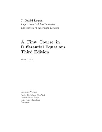
1.1 First-Order Equations7to the amount present; r denotes the proportionality constant and in thefollowing discussion we assume it is a fixed number. Although it is easy toguess a solution to this equation, we want to solve it from basic principles. Werewrite the equation asx′ r,xand then observe from the chain rule thatx′d ln x.xdtThus the equation becomesdln x r.dtRemembering that x is a function of t, we integrate both sides with respect tot to getZZdln x dt r dt.dtThe integral of the derivative of a function is the function itself (integrationand differentiation are inverse processes), and so we getln x rt C1 ,where C1 is an arbitrary constant of integration. Solving for x givesx e rt C1 eC1 e rt Ce rt ,where C is an arbitrary constant which can take on any value. (Note: if C1 isan arbitrary constant, then C eC1 must also be arbitrary.) Therefore, thereare infinitely many solutions to the decay equation (1.4) given byx(t) Ce rt .(1.5)The infinite set of solutions (1.5) of a first-order equation is called the generalsolution of the equation. The general solution contains an arbitrary constantC, and as such it is also referred to as a one-parameter family of solutions—one for each choice of C. They are also referred to as the integral curves ofthe differential equation. These curves are plotted in Figure 1.2. One can askhow there can be infinitely many solutions to a decay problem. In a real systemthere is typically an initial condition imposed on the state x(t); that is,x(0) x0 ,(initial condition)where x0 is a prescribed, fixed state at time t 0. This initial condition picksout a specific value of the arbitrary constant C, and hence a specific solution

81. First-Order Differential EquationsxxC 1x0C 0.5ttC -0.5C -1Figure 1.2 (Left) Plots of four integral curves, or solution curves (1.5), of thedifferential equation (1.4), for four values of C. (Right) A particular solutionsatisfying the initial condition x(0) x0 .curve. In this case, x(0) x0 C exp( r · 0) C. Therefore we have selectedout a particular solutionx(t) x0 e rtof the DE (1.4). To repeat, of the many solutions, we have chosen the one thatsatisfies the

equations; equilibrium solutions, stability and bifurcation. Other special types of equations, for example, Bernoulli, exact, and homogeneous equa-tions, are covered in the Exercises with generous guidance. Many applica-tions are discussed from science, engineering, economics, and biology. Chapter 2. Second-order linear equations.