Transcription
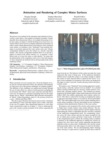
Animation and Rendering of Complex Water SurfacesDouglas EnrightStanford UniversityIndustrial Light & Magicenright@stanford.eduStephen MarschnerStanford Universitysrm@graphics.stanford.eduRonald FedkiwStanford UniversityIndustrial Light & Magicfedkiw@cs.stanford.eduAbstractWe present a new method for the animation and rendering of photorealistic water effects. Our method is designed to produce visuallyplausible three dimensional effects, for example the pouring of water into a glass (see figure 1) and the breaking of an ocean wave, in amanner which can be used in a computer animation environment. Inorder to better obtain photorealism in the behavior of the simulatedwater surface, we introduce a new “thickened” front tracking technique to accurately represent the water surface and a new velocityextrapolation method to move the surface in a smooth, water-likemanner. The velocity extrapolation method allows us to provide adegree of control to the surface motion, e.g. to generate a windblown look or to force the water to settle quickly. To ensure thatthe photorealism of the simulation carries over to the final images,we have integrated our method with an advanced physically basedrendering system.CR Categories: I.3.7 [Computer Graphics]: Three-DimensionalGraphics and Realism—Animation; I.3.7 [Computer Graphics]:Three-Dimensional Graphics and Realism—Raytracing;Keywords: computational fluid dynamics, implicit surfaces, natural phenomena, physically based animation, rendering, volume rendering1IntroductionWater surrounds us in our everyday lives. Given the ubiquity of water and our constant interaction with it, the animation and renderingof water poses one of the greatest challenges in computer graphics.The difficulty of this challenge was underscored recently throughthe use of water effects in a variety of motion pictures including therecent feature film “Shrek” where water, mud, beer and milk effectswere seen. In response to a question concerning what was the singlehardest shot in “Shrek”, DreamWorks SKG principal and producerof “Shrek”, Jeffrey Katzenberg, stated, It’s the pouring of milk intoa glass. [Hiltzik and Pham 2001].The above quote illustrates the need for photorealistic simulationand rendering of water (and other liquids such as milk), especiallyin the case of complex, three dimensional behavior as seen whenwater is poured into a glass as in figure 1. A key to achieving thisgoal is the visually accurate treatment of the surface separating theFigure 1: Water being poured into a glass (55x120x55 grid cells).water from the air. The behavior of this surface provides the visualimpression that water is being seen. If the numerical simulationmethod used to model this surface is not robust enough to capturethe essence of water, then the effect is ruined for the viewer. A variety of new techniques for treatment of the surface are proposed inthis paper in order to provide visually pleasing motion and photorealistic results.We propose a new “thickened” front tracking approach to modeling the surface, called the ”particle level set method”. It is a hybridsurface tracking method that uses massless marker particles combined with a dynamic implicit surface. This method was entirelyinspired by the hybrid liquid volume model proposed in [Foster andFedkiw 2001], but exhibits significantly more realistic surface behavior. This effect is achieved by focusing on modeling the surfaceas opposed to the liquid volume as was done by [Foster and Fedkiw2001]. This shift in philosophy away from volume modeling and towards surface modeling, is the key idea behind our new techniques,resulting in better photorealistic behavior of the water surface.We propose a new treatment of the velocity at the surface in orderto obtain more visually realistic water surface behavior. The motion of both the massless marker particles and the implicit functionrepresenting the surface is dependent upon the velocities containedon the underlying computational mesh. By extrapolating velocities across the water surface and into the region occupied by theair, we obtain more accurate and better visual results. In the limitas the computational grid is refined, the resulting surface conditionis identical to the traditional approach of making the velocity divergence free, but it gives more visually appealing and physicallyplausible results on coarse grids. Furthermore, this velocity extrapolation procedure allows us to add a degree of control to the behavior of the water surface. We can add dampening and/or churningeffects forcing it to quiet down or splash up faster than would be
allowed by a straightforward physical simulation.Our new advances can be easily incorporated into a pre-existingNavier-Stokes solver for water. In fact, we solve the Navier-Stokesequations for liquid water along the lines of [Foster and Fedkiw2001], in particular using a semi-Lagrangian “stable fluid” approach introduced to the community by Stam [Stam 1999]. Ourapproach preserves as much of the realistic behavior of the wateras possible, while at the same time providing a degree of controlnecessary for its use in a computer animation environment.Photorealistic rendering is necessary in order to complete thecomputational illusion of real water. In some ways water is an easymaterial to render, because unlike many common materials its optical properties are well understood and are easy to describe. In allbut the largest-scale scenes, surface tension prevents water surfacesfrom exhibiting the microscopic features that make reflection frommany other materials so complicated. However, water invariablycreates situations in which objects are illuminated through complexrefracting surfaces, which means that the light transport problemthat is so easy to state is difficult to solve. Most widely used rendering algorithms disregard this sort of illumination or handle it usingsimple approximations, but because water and its illumination effects are so familiar these approaches fail to achieve realism. Thereare several rendering algorithms that can properly account for alltransport paths, including the illumination through the water surface; some examples are path tracing [Kajiya 1986], bidirectionalpath tracing [Heckbert 1990; Lafortune and Willems 1993; Veachand Guibas 1994], Metropolis light transport [Veach and Guibas1997], and photon mapping [Jensen 1995]. In our renderings ofclear water for this paper we have chosen photon mapping becauseit is simple and it makes it easy to avoid the distracting noise thatoften arises in pure path sampling algorithms from illuminationthrough refracting surfaces.2Previous WorkEarly (and continuing) work by the graphics community into themodeling of water phenomenon focused on reduced model representations of the water surface, ranging from Fourier synthesismethods [Masten et al. 1987] to parametric representations of thewater surface [Schachter 1980; Fournier and Reeves 1986; Peachey1986; Ts’o and Barsky 1987]. The last three references are notablein the way they attempt to model realistic wave behavior includingthe change in wave behavior as a function of the depth of the water.Fairly realistic two dimensional wave scenery can be developed using these methods including the illusion of breaking waves, but ultimately they are all constrained by the sinusoidal modeling assumption present in each of them. They are unable to easily deal withcomplex three dimensional behaviors such as flow around objectsand dynamically changing boundaries. A summary of the abovemethods and their application to modeling and rendering of oceanwave environments can be found in [Tessendorf 2001].In order to obtain water models which could potentially be usedin a dynamic animation environment, researchers turned towardsusing two dimensional approximations to the full 3D Navier-Stokesequations. [Kass and Miller 1990] use a linearized form of the 2Dshallow water equations to obtain a height field representation ofthe water surface. A pressure defined height field formulation wasused by [Chen and Lobo 1994] in fluid simulations with movingobstacles. [O’Brien and Hodgins 1995] used a height model combined with a particle system in order to simulate splashing liquids.The use of a height field gives a three dimensional look to a twodimensional flow calculation, but it constrains the surface to be afunction, i.e. the surface passes the vertical line test where for each(x,y) position there is at most one z value. The surface of a crashing wave or of water being poured into a glass does not satisfy thevertical line test. Use of particle systems permits the surface tobecome multivalued. A viscous spring particle representation of aliquid has been proposed by [Miller and Pearce 1989]. An alternative molecular dynamics approach to the simulation of particles inthe liquid phase has been developed by [Terzopoulos et al. 1989].Particle methods, while quite versatile, can pose difficulties whentrying to reconstruct a smooth water surface from the locations ofthe particles alone.The simulation of complex water effects using the full 3DNavier-Stokes equations has been based upon the large amount ofresearch done by the computational fluid dynamics community overthe past 50 years. [Foster and Metaxas 1996] utilized the workof [Harlow and Welch 1965] in developing a 3D Navier-Stokesmethodology for the realistic animation of liquids. Further CFDenhancements to the traditional marker and cell method of Harlow and Welch which allow one to place particles only near thesurface can be found in [Chen et al. 1997]. A semi-Lagrangian”stable fluids” treatment of the convection portion of the NavierStokes equations was introduced to the computer graphics community by [Stam 1999] in order to allow the use of significantlylarger time steps without hindering stability. [Foster and Fedkiw2001] made significant contributions to the simulation and controlof three dimensional fluid simulations through the introduction of ahybrid liquid volume model combining implicit surfaces and massless marker particles; the formulation of plausible boundary conditions for moving objects in a liquid; the use of an efficient iterative method to solve for the pressure; and a time step subcyclingscheme for the particle and implicit surface evolution equations inorder to reduce the amount of visual error inherent to the large semiLagrangian “stable fluid” time step used for time evolving the fluidvelocity and the pressure. The combination of all of the above advances in 3D fluid simulation technology along with ever increasingcomputational resources has set the stage for the inclusion of fully3D fluid animation tools in a production environment.Most work on simulating water at small scales has not specifically addressed rendering and has not used methods that correctlyaccount for all significant light transport paths. Research on therendering of illumination through water [Watt 1990; Nishita andNakamae 1994] has used methods based on processing each polygon of a mesh that represents a fairly smooth water surface, sothese methods cannot be used for the very complex implicit surfaces that result from our simulations. For the case of 2D wavefields in the open ocean, approaches motivated by physical correctness have produced excellent results [Premoze and Ashikhmin2000; Tessendorf 2001].33.1Simulation MethodMotivation[Foster and Fedkiw 2001] chose to define the liquid volume being simulated as one side of an isocontour of an implicit function,φ . The surface of the water was defined by the φ 0 isocontourwith φ 0 representing the water and φ 0 representing the air.By using an implicit function representation of the liquid volume,they obtained a smooth, temporally coherent liquid surface. Theyrejected the use of particles alone to represent the liquid surface because it is difficult to a calculate a visually desirable smooth liquidsurface from the discrete particles alone. The implicit surface wasdynamically evolved in space and time according to the underlying liquid velocity u. As shown in [Osher and Sethian 1988], theappropriate equation to do this isφt u · φ 0(1)where φt is the partial derivative of φ with respect to time and ( / x, / y, / z) is the gradient operator.
An implicit function only approach to modeling the surface willnot yield realistic surface behavior due to an excessive amount ofvolume loss on coarse grids. A seminal advance of [Foster andFedkiw 2001] in creating realistic liquids for computer animationis the hybridization of the visually pleasing smooth implicit function modeling of the liquid volume with particles that can maintainthe liquid volume on coarse grids. The inclusion of particles provides a way for capturing the liveliness of a real liquid with sprayand splashing effects. Curvature was used as an indicator for allowing particles to influence the implicit surface representation of thewater. This is a natural choice since small droplets of water havevery high curvature and dynamic implicit surfaces have difficultyresolving features with sharp corners.Figure 2(a) shows a notched disk that we rotate for one rigidbody rotation about the point (50,50). The inside of the disk canbe thought of as a volume of liquid. Figure 2(b) shows the result of using an implicit surface only approach (after one rotation)where both the higher and lower corners of the disk are erroneouslyshaved off causing both loss of visual features and an artificiallyviscous look for the liquid. This numerical result was obtained using a highly accurate fifth order WENO discretization of equation1 (see e.g. [Jiang and Peng 2000; Osher and Fedkiw 2002]). Forthe sake of comparison, we note that [Sethian 1999] only proposessecond order accurate methods for discretizing this equation. Figure 2(c) shows the result obtained with our implementation of themethod from [Foster and Fedkiw 2001]. The particles inside thedisk do not allow the implicit surface to cross over them and helpto preserve the two corners near the bottom. However, there is little they can do to stop the implicit surface from drifting away fromthem near the top corners. This represents loss of air or bubbles asthe method erroneously gains liquid volume. This is not desirablesince many complex water motions such as wave phenomenon aredue in part to differing heights of water columns adjacent to eachother. Loss of air in a water column reduces the pressure forcesfrom neighboring columns destroying many of the dynamic splashing effects as well as the overall visually stimulating liveliness ofthe liquid.While the hybrid liquid volume model of Foster and Fedkiw attempts to maintain the volume of the liquid accurately, it fails tomodel the air or more generally the opposite side of the liquid surface. We shift the focus away from maintaining a liquid volumetowards maintaining the liquid surface itself. An immediate advantage of this approach is that it leads to symmetry in particle placement. We place particles on both sides of the surface and use themto maintain an accurate representation of the surface itself regardless of what may be on one side or the other. The particles are notmeant to track volume, they are intended to correct errors in thesurface representation by the implicit function. In [Enright et al.2002] we showed that this surface only approach leads to the mostaccurate 3D results for surface tracking ever achieved (in both CFDand CG). This was done for analytical ”test” velocity fields. Figure 2(d) shows that this new method correctly computes the rigidbody rotation for the notched disk preserving both the water andthe air volumes so that more realistic water motion can be obtained.In this current paper, we couple this new method to real velocityfields and fluid dynamics calculations for the first time. Representative results of this new method can be seen in figure 3. A ballis thrown into a tank of water with the same tank geometry, gridspacing and ball speed as seen in figure 4 (courtesy of [Foster andFedkiw 2001]). The resulting splash after the ball impacts the surface of the water is dramatically different between the two figures.Our new method produces the well formed, thin sheet one wouldvisually expect. Note that the distorted look of the ball in our figure is due to the correct calculation of the refraction of light whenit passes through the surface of the water. To give an indicationof the additional computational cost incurred using our new simu-(a) Initial Notched Disk(b) Implicit Surface Only(c) Particles Inside Only(d) Our New MethodFigure 2: Rigid Body Rotation Testlation method, figure 3 took about 11 minutes per frame, figure 4took about 7 minutes per frame and a level set only solution takesabout 3 minutes per frame. The rendering time for figure 3 wasapproximately 15 minutes per frame.3.23.2.1Particle Level Set MethodInitialization of ParticlesTwo sets of particles are randomly placed in a “thickened” surfaceregion (we use three grid cells on each side of the surface) withpositive particles in the φ 0 region and negative particles in theφ 0 region. There is no need to place particles far away fromthe surface since the sign of the level set function readily identifiesthese regions gaining large computational savings. The number ofparticles placed in each cell is an adjustable parameter that can beused to control the amount of resolution, e.g. we use 64 particlesper cell for most of our examples. Each particle possesses a radius,r p , which is constrained to take a minimum and maximum valuebased upon the size of the underlying computational cells used inthe simulation. A minimum radius of .1 min( x, y, z) and maximum radius of .5 min( x, y, z) appear to work well. The radiusof a particle changes dynamically throughout the simulation, sincea particle’s location relative to the surface changes. The radius isset according to: rmaxif s p φ ( x p ) rmaxs p φ ( x p ) if rmin s p φ ( x p ) rmax ,rp (2) rif s p φ ( x p ) rminminwhere s p is the sign of the particle ( 1 for positive particles and-1 for negative particles). This radius adjustment keeps the boundary of the spherical particle tangent to the surface whenever possible. This fact combined with the overlapping nature of the particle
Figure 3: Our New Method (140x110x90 grid cells).Figure 4: Foster and Fedkiw 2001 (140x110x90 grid cells).spheres allows for an enhanced reconstruction capability of the liquid surface.negative particles. The result is an improved representation of thesurface of the liquid.3.2.23.2.4Time IntegrationThe marker particles and the implicit function are separately integrated forward in time using a forward Euler time integrationscheme. The implicit function is integrated forward using equation 1, while the particles are passively advected with the flow using d x p /dt u p , where u p is the fluid velocity interpolated to theparticle position x p .3.2.3Error Correction of the Implicit SurfaceIdentification of Error: The main role of the particles is to detect when the implicit surface has suffered inaccuracies due to thecoarseness of the computational grid in regions with sharp features.Particles that are on the wrong side of the interface by more thantheir radius, as determined by a locally interpolated value of φ atthe particle position x p , are considered to have escaped their sideof the interface. This indicates errors in the implicit surface representation. In smooth, well resolved regions of the interface, ourdynamic implicit surface is highly accurate and particles do not drifta non-trivial distance across the interface.Quantification of Error: We associate a spherical implicit function , designated φ p , with each particle p whose size is determinedby the particle radius, i.e.φ p ( x) s p (r p x x p ).(3)Any difference in φ from φ p indicates errors in the implicit functionrepresentation of the surface. That is, the implicit version of thesurface and the particle version of the surface disagree.Error Correction: We use escaped positive particles to rebuildthe φ 0 region and escaped negative particles to rebuild the φ 0region as defined by the implicit function. The reconstruction of theimplicit surface occurs locally within the cell that each escaped particle currently occupies. Using equation 3, the φ p values of escapedparticles are calculated for the eight grid points on the boundary ofthe cell containing the particle. This value is compared to the current value of φ for each grid point and we take the smaller value(in magnitude) which is the value closest to the φ 0 isocontourdefining the surface. We do this for all escaped positive and escapedWhen To Apply Error CorrectionWe apply the error correction method discussed above after anycomputational step in which φ has been modified in some way.This occurs when φ is integrated forward in time and when theimplicit function is smoothed to obtain a visually pleasing surface.We smooth the implicit surface with an equation of the formφτ S(φτ 0 )( φ 1),(4)where τ is a fictitious time and S(φ ) is a smoothed signed distancefunction given byφS(φ ) pφ 2 ( x)2.(5)More details on this are given in [Foster and Fedkiw 2001].3.2.5Particle ReseedingIn complex flows, a liquid interface can be stretched and torn in adynamic fashion. The use of only an initial seeding of particles willnot capture these effects well, as regions will form that lack a sufficient number of particles to adequately perform the error correctionstep. Periodically, e.g. every 20 frames, we randomly reseed particles about the “thickened” interface to avoid this dilemma. Thisis done by randomly placing particles near the interface, and thenusing geometric information contained within the implicit function(e.g. the direction of the shortest possible path to the surface isgiven by N φ / φ ) to move the particles to their respectivedomains, φ 0 or φ 0. The goal of this reseeding step is to preserve the initial particle resolution of the interface, e.g. 64 particlesper cell. Thus, if a given cell has too few or too many particles,some can be added or deleted respectively.3.2.6A Note on Alternative MethodsIf we felt that preserving the volume of the fluid was absolutely necessary in order to obtain visually pleasing fluid behavior, we wouldhave chosen to use a volume of fluid (VOF) [Hirt and Nichols 1981]representation of the fluid. Although VOF methods explicitly conserve volume, they produce visually disturbing artifacts allowingthin liquid sheets to artificially break up and form “blobbies” and
“flotsam” of liquid. Also, a visually desirable smooth fluid interfaceis difficult to construct when using these methods.Another alternative is to explicitly discretize the free surface withparticles and maintain a connectivity list between particles, see e.g.[Unverdi and Tryggvason 1992]. This connectivity list is difficultto maintain when parts of the free surface break apart or mergetogether as is often seen in complex flows of water and other liquids.Our approach avoids the especially difficult issues associated withmaintaining particle connectivity information.3.3Velocities at the SurfaceAlthough the Navier-Stokes equations can be used to find the velocity within the liquid volume, boundary conditions are needed forthe velocity on the air side near the free surface. These boundarycondition velocities are used in updating the Navier-Stokes equations, moving the surface, and moving the particles placed near thesurface. The velocity at the free surface of the water can be determined through the usual enforcement of the conservation of mass(volume) constraint, · u 0, where u (u, v, w) is the velocity ofthe liquid. This equation allows us to determine the velocities onall the faces of computational cells that contain the φ 0 isocontour. Unfortunately, the procedure for doing this is not unique whenmore than one face of a cell needs a boundary condition velocity. Avariety of methods have been proposed, e.g. see [Chen et al. 1995]and [Foster and Metaxas 1996].We propose a different approach altogether, the extrapolation ofthe velocity across the surface into the surrounding air. As the computational grid is refined, this method is equivalent to the usualmethod, but it gives a smoother and more visually pleasing motionof the surface on coarser (practical sized) grids. We extrapolate thevelocity out a few grid cells into the air, obtaining boundary condition velocities in a band of cells on the air side of the surface. Thisallows us to use higher order accurate methods and obtain betterresults when moving the implicit surface using equation 1 and alsoprovides velocities for updating the position of particles on the airside of the surface. Velocity extrapolation also assists in the implementation of the semi-Lagrangian “stable fluid” method, since thereare times when characteristics generated by this approach look backacross the interface (a number of cells) into the air region for validvelocities.3.3.1proceed to the next point corresponding to the next smallest valueof φ , etc. Further details of this method are discussed in [Adalsteinsson and Sethian 1999].3.3.2Velocity AdvectionThe momentum portion of the Navier-Stokes equations is: ut u · u ν · ( u) 3.3.3ControlOur velocity extrapolation method enables us to apply a newly devised method for controlling the nature of the surface motion. Thisis done simply by modifying the extrapolated velocities on the airside of the surface. For example, to model wind-blown water as aresult of air drag, we take a convex combination of the extrapolatedvelocities with a pre-determined wind velocity field u (1 α) uext α uwind ,The equation modeling this extrapolation for the x component ofthe velocity, u, is given by(6)where N (nx , ny , nz ) is a unit vector perpendicular to the implicitsurface and τ is fictitious time. A similar equation holds for thev and w components of velocity field. Since we use an implicitsurface to describe the fluid, N φ / φ . Fast methods exist forsolving this equation in O(n log n) time, where n is the number ofgrid points that one needs to extrapolate over, in our case a five gridcell thick band on the air side of the interface. The fast method isbased upon the observation that information in equation 6 propagates in only one direction away from the surface. This implies thatwe do not have to revisit previously computed values of uext (theextrapolated velocity) if we perform the calculation in the correctorder. The order is determined by the value of φ allowing us todo an O(n log n) sorting of the points before beginning the calculation. The value of u itself is determined by enforcing the conditionat steady state, namely φ · u 0 where the derivatives are determined using previously calculated values of φ and u. From thisscalar equation, a new value of u can be determined, and then we(7)where ν is the kinematic viscosity of the fluid, ρ is the density ofthe fluid, p is the pressure, and g is an externally applied gravityfield. We use the semi-Lagrangian “stable fluids” method [Stam1999] to update the convective portion of this equation, i.e. the u · u term. This method calculates the first term on the left handside of equation 7 by following the fluid characteristics backwardsin time to determine from which computational cell the volume offluid came, and then taking an average of the appropriate velocities there. This allows one to stably take much larger time stepsthan would be allowed using other time advancement schemes forvelocity advection. A consequence of the now allowed large semiLagrangian time step is that near the surface, we might look acrossthe interface as many as a few grid cells into the air region to findvelocities. In a standard approach, valid velocities are not definedin this region. However, our velocity extrapolation technique easilyhandles this case ensuring that physically plausible velocities exist afew grid cells into the air region. In fact, we extrapolate the velocitythe maximum distance from the surface that would be allowed during a semi-Lagrangian ”stable fluids” time step guaranteeing that asmooth, physically plausible and visually appealing velocity can befound there.Extrapolation Method u N · u, τ1 p g,ρ(8)where uext is the extrapolated velocity, uwind a desired air-like velocity, and 0 α 1 the mixing constant. This can be appliedthroughout the surface or only locally in select portions of the computational domain as desired. Note that setting uwind 0 forceschurning water to settle down faster with the fastest settling resulting from α 1. All of the figures shown in the paper used α 0,but we demonstrate how α can be used to force a poured glass ofwater to settle more quickly in the accompanying video.3.4SummaryWe divide up the computational domain into voxels with the components of u stored on the appropriate faces and p, ρ and φ storedat the center of each cell. This arrangement of computational variables is the classic staggered MAC-style arrangement [Harlow andWelch 1965]. The density of a given cell is given by the value of φat the center of the cell. The evolution of u, p, ρ and φ in a giventime step is performed in a series of three steps as outlined below:1. The current surface velocity is smoothly extrapolated acrossthe surface into the air region as discussed in section 3.3.1.Appropriate control behavior modifications to the velocityfield are made.
2. The water surface and marker particles are integrated forwardin time via an explicit time step subcycling method with theappropriate corrections to φ as described in section 3.2.3.3. The velocity field is updated with equation 7 using the updated values for ρ. This is done by first using the semiLagrangian “stable fluid” method to find an estimate for thevelocity. This estimate i
Stephen Marschner Stanford University srm@graphics.stanford.edu Ronald Fedkiw Stanford University Industrial Light & Magic fedkiw@cs.stanford.edu Abstract We present a new method for the animation and rendering of photo-realistic water effects. Our method is designed to produce visually plausible three dimensional effects, for example the .