Transcription
CHAPTER 7: OPTIMAL RISKY PORTFOLIOSCHAPTER 7: OPTIMAL RISKY PORTFOLIOSPROBLEM SETS1.(a) and (e).2.(a) and (c). After real estate is added to the portfolio, there are four asset classes in the portfolio:stocks, bonds, cash and real estate. Portfolio variance now includes a variance term for real estatereturns and a covariance term for real estate returns with returns for each of the other three assetclasses. Therefore, portfolio risk is affected by the variance (or standard deviation) of real estatereturns and the correlation between real estate returns and returns for each of the other assetclasses. (Note that the correlation between real estate returns and returns for cash is most likelyzero.)3.(a) Answer (a) is valid because it provides the definition of the minimum variance portfolio.4.The parameters of the opportunity set are:E(rS) 20%, E(rB) 12%, σS 30%, σB 15%, ρ 0.10From the standard deviations and the correlation coefficient we generate the covariance matrix[note that C o v ( rS , rB ) S B ]:BondsStocksBonds22545Stocks45900The minimum-variance portfolio is computed as follows: B Cov ( r S , r B )2wMin(S) S B 2 Cov ( r S , r B )22 225 45900 225 ( 2 45 ) 0 . 1739wMin(B) 1 0.1739 0.8261The minimum variance portfolio mean and standard deviation are:E(rMin) (0.1739 .20) (0.8261 .12) .1339 13.39%σMin [w S S w222B 2B 2w SwBCov ( r S , r B )]1/2 [(0.17392 900) (0.82612 225) (2 0.1739 0.8261 45)]1/2 13.92%7-1
CHAPTER 7: OPTIMAL RISKY PORTFOLIOS5.Proportionin stock 0%Proportionin bond 5.70%16.54%19.53%24.48%30.00%minimum variancetangency portfolioGraph shown below.25.00INVESTMENT OPPORTUNITY SETCML20.00TangencyPortfolioEfficient frontierof risky assets15.00MinimumVariancePortfolio10.00rf 8.005.000.000.006.5.0010.0015.0020.0025.0030.00The above graph indicates that the optimal portfolio is the tangency portfolio with expected returnapproximately 15.6% and standard deviation approximately 16.5%.7-2
CHAPTER 7: OPTIMAL RISKY PORTFOLIOS7.The proportion of the optimal risky portfolio invested in the stock fund is given by:wS [ E ( rS ) r f ] [ E ( rS ) r f ] 2B2B [ E ( r B ) r f ] C o v ( rS , r B ) [ E ( rB ) r f ] 2S [ E ( rS ) r f E ( r B ) r f ] C o v ( r S , r B )[(.2 0 .0 8 ) 2 2 5 ] [(.1 2 .0 8 ) 4 5 ][(.2 0 .0 8 ) 2 2 5 ] [(.1 2 .0 8 ) 9 0 0 ] [(.2 0 .0 8 .1 2 .0 8 ) 4 5 ] 0 .4 5 1 6w B 1 0 .4 5 1 6 0 .5 4 8 4The mean and standard deviation of the optimal risky portfolio are:E(rP) (0.4516 .20) (0.5484 .12) .1561 15.61%σp [(0.45162 900) (0.54842 225) (2 0.4516 0.5484 45)]1/2 16.54%8.The reward-to-volatility ratio of the optimal CAL is:E ( rp ) r f 9.a. p.1 5 6 1 .0 8 0 .4 6 0 1 .4601should be .4603 (rounding).1 6 5 4If you require that your portfolio yield an expected return of 14%, then you can find thecorresponding standard deviation from the optimal CAL. The equation for this CAL is:E ( rC ) r f E ( rp ) r f C .0 8 0 .4 6 0 1 C.4601 should be .4603 (rounding)PIf E(rC) is equal to 14%, then the standard deviation of the portfolio is 13.03%.b.To find the proportion invested in the T-bill fund, remember that the mean of the completeportfolio (i.e., 14%) is an average of the T-bill rate and the optimal combination of stocks andbonds (P). Let y be the proportion invested in the portfolio P. The mean of any portfolioalong the optimal CAL is:E ( rC ) (1 y ) r f y E ( rP ) r f y [ E ( rP ) r f ] .0 8 y ( .1 5 6 1 .0 8 )Setting E(rC) 14% we find: y 0.7881 and (1 y) 0.2119 (the proportion invested in theT-bill fund).To find the proportions invested in each of the funds, multiply 0.7884 times the respectiveproportions of stocks and bonds in the optimal risky portfolio:Proportion of stocks in complete portfolio 0.7881 0.4516 0.3559Proportion of bonds in complete portfolio 0.7881 0.5484 0.43227-3
CHAPTER 7: OPTIMAL RISKY PORTFOLIOS10.Using only the stock and bond funds to achieve a portfolio expected return of 14%, we must findthe appropriate proportion in the stock fund (wS) and the appropriate proportion in the bond fund(wB 1 wS) as follows:.14 .20 wS .12 (1 wS) .12 .08 wS wS 0.25So the proportions are 25% invested in the stock fund and 75% in the bond fund. The standarddeviation of this portfolio will be:σP [(0.252 900) (0.752 225) (2 0.25 0.75 45)]1/2 14.13%This is considerably greater than the standard deviation of 13.04% achieved using T-bills and theoptimal portfolio.11.a.Even though it seems that gold is dominated by stocks, gold might still be an attractive asset tohold as a part of a portfolio. If the correlation between gold and stocks is sufficiently low, goldwill be held as a component in a portfolio, specifically, the optimal tangency portfolio.7-4
CHAPTER 7: OPTIMAL RISKY PORTFOLIOSb.12.If the correlation between gold and stocks equals 1, then no one would hold gold. The optimalCAL would be comprised of bills and stocks only. Since the set of risk/return combinations ofstocks and gold would plot as a straight line with a negative slope (see the following graph),these combinations would be dominated by the stock portfolio. Of course, this situation couldnot persist. If no one desired gold, its price would fall and its expected rate of return wouldincrease until it became sufficiently attractive to include in a portfolio.Since Stock A and Stock B are perfectly negatively correlated, a risk-free portfolio can be createdand the rate of return for this portfolio, in equilibrium, will be the risk-free rate. To find theproportions of this portfolio [with the proportion wA invested in Stock A and wB (1 – wA )invested in Stock B], set the standard deviation equal to zero. With perfect negative correlation,the portfolio standard deviation is:σP Absolute value [wAσA wBσB]0 5 wA [10 (1 – wA)] wA 0.6667The expected rate of return for this risk-free portfolio is:E(r) (0.6667 10) (0.3333 15) 11.667%Therefore, the risk-free rate is: 11.667%13.False. If the borrowing and lending rates are not identical, then, depending on the tastes of theindividuals (that is, the shape of their indifference curves), borrowers and lenders could havedifferent optimal risky portfolios.7-5
CHAPTER 7: OPTIMAL RISKY PORTFOLIOS14.False. The portfolio standard deviation equals the weighted average of the component-assetstandard deviations only in the special case that all assets are perfectly positively correlated.Otherwise, as the formula for portfolio standard deviation shows, the portfolio standard deviationis less than the weighted average of the component-asset standard deviations. The portfoliovariance is a weighted sum of the elements in the covariance matrix, with the products of theportfolio proportions as weights.15.The probability distribution is:Probability0.70.3Rate of Return100% 50%Mean [0.7 100%] [0.3 (-50%)] 55%Variance [0.7 (100 55)2] [0.3 (-50 55)2] 4725Standard deviation 47251/2 68.74%16.σP 30 y σ 40 y y 0.75E(rP) 12 0.75(30 12) 25.5%17.The correct choice is c. Intuitively, we note that since all stocks have the same expected rate ofreturn and standard deviation, we choose the stock that will result in lowest risk. This is the stockthat has the lowest correlation with Stock A.More formally, we note that when all stocks have the same expected rate of return, the optimalportfolio for any risk-averse investor is the global minimum variance portfolio (G). When theportfolio is restricted to Stock A and one additional stock, the objective is to find G for any pairthat includes Stock A, and then select the combination with the lowest variance. With two stocks,I and J, the formula for the weights in G is: J Cov ( r I , r J )2wMin(I) wMin(J) 1 w I J 2 Cov ( r I , r J )22Min(I)Since all standard deviations are equal to 20%:C o v ( rI , r J ) I J 4 0 0 a n d w M in ( I ) w M in ( J ) 0 .5This intuitive result is an implication of a property of any efficient frontier, namely, that thecovariances of the global minimum variance portfolio with all other assets on the frontier areidentical and equal to its own variance. (Otherwise, additional diversification would further reducethe variance.) In this case, the standard deviation of G(I, J) reduces to: M in( G ) [ 2 0 0 (1 I J ) ]1/ 2This leads to the intuitive result that the desired addition would be the stock with the lowest7-6
CHAPTER 7: OPTIMAL RISKY PORTFOLIOScorrelation with Stock A, which is Stock D. The optimal portfolio is equally invested in Stock Aand Stock D, and the standard deviation is 17.03%.18.No, the answer to Problem 17 would not change, at least as long as investors are not risk lovers.Risk neutral investors would not care which portfolio they held since all portfolios have anexpected return of 8%.19.Yes, the answers to Problems 17 and 18 would change. The efficient frontier of risky assets ishorizontal at 8%, so the optimal CAL runs from the risk-free rate through G. This implies riskaverse investors will just hold Treasury Bills.20.Rearranging the table (converting rows to columns), and computing serial correlation results inthe following table:Nominal 7.745.022.93Serial Correlation0.46-0.220.600.590.630.23For example: to compute serial correlation in decade nominal returns for large-company stocks, weset up the following two columns in an Excel spreadsheet. Then, use the Excel function“CORREL” to calculate the correlation for the 1.25%9.11%19.41%7.84%5.90%17.60%Note that each correlation is based on only seven observations, so we cannot arrive at anystatistically significant conclusions. Looking at the results, however, it appears that, with theexception of large-company stocks, there is persistent serial correlation. (This conclusion changeswhen we turn to real rates in the next problem.)7-7
CHAPTER 7: OPTIMAL RISKY PORTFOLIOS21.The table for real rates (using the approximation of subtracting a decade’s average inflation fromthe decade’s average nominal return) is:Real 4.99-0.351.37-1.073.902.09Serial Correlation0.29-0.270.380.110.00While the serial correlation in decade nominal returns seems to be positive, it appears that realrates are serially uncorrelated. The decade time series (although again too short for any definitiveconclusions) suggest that real rates of return are independent from decade to decade.7-8
CHAPTER 7: OPTIMAL RISKY PORTFOLIOSCFA PROBLEMS1.a.Restricting the portfolio to 20 stocks, rather than 40 to 50 stocks, will increase the risk of theportfolio, but it is possible that the increase in risk will be minimal. Suppose that, for instance,the 50 stocks in a universe have the same standard deviation ( ) and the correlations betweeneach pair are identical, with correlation coefficient ρ. Then, the covariance between each pair ofstocks would be ρσ2, and the variance of an equally weighted portfolio would be: P 21n 2 n 1 2nThe effect of the reduction in n on the second term on the right-hand side would berelatively small (since 49/50 is close to 19/20 and ρσ2 is smaller than σ2), but thedenominator of the first term would be 20 instead of 50. For example, if σ 45% and ρ 0.2, then the standard deviation with 50 stocks would be 20.91%, and would rise to 22.05%when only 20 stocks are held. Such an increase might be acceptable if the expected return isincreased sufficiently.Hennessy could contain the increase in risk by making sure that he maintains reasonablediversification among the 20 stocks that remain in his portfolio. This entails maintaining alow correlation among the remaining stocks. For example, in part (a), with ρ 0.2, theincrease in portfolio risk was minimal. As a practical matter, this means that Hennessywould have to spread his portfolio among many industries; concentrating on just a fewindustries would result in higher correlations among the included stocks.2.Risk reduction benefits from diversification are not a linear function of the number of issues in theportfolio. Rather, the incremental benefits from additional diversification are most important whenyou are least diversified. Restricting Hennessy to 10 instead of 20 issues would increase the risk ofhis portfolio by a greater amount than would a reduction in the size of the portfolio from 30 to 20stocks. In our example, restricting the number of stocks to 10 will increase the standard deviationto 23.81%. The 1.76% increase in standard deviation resulting from giving up 10 of 20 stocks isgreater than the 1.14% increase that results from giving up 30 of 50 stocks.3.The point is well taken because the committee should be concerned with the volatility of the entireportfolio. Since Hennessy’s portfolio is only one of six well-diversified portfolios and is smallerthan the average, the concentration in fewer issues might have a minimal effect on thediversification of the total fund. Hence, unleashing Hennessy to do stock picking may beadvantageous.4.d.5.c.Portfolio Y cannot be efficient because it is dominated by another portfolio. For example,Portfolio X has both higher expected return and lower standard deviation.7-9
CHAPTER 7: OPTIMAL RISKY PORTFOLIOS6.d.7.b.8.a.9.c.10.Since we do not have any information about expected returns, we focus exclusively on reducingvariability. Stocks A and C have equal standard deviations, but the correlation of Stock B with Stock C(0.10) is less than that of Stock A with Stock B (0.90). Therefore, a portfolio comprised of Stocks B andC will have lower total risk than a portfolio comprised of Stocks A and B.11.Fund D represents the single best addition to complement Stephenson's current portfolio, given hisselection criteria. Fund D’s expected return (14.0 percent) has the potential to increase theportfolio’s return somewhat. Fund D’s relatively low correlation with his current portfolio ( 0.65)indicates that Fund D will provide greater diversification benefits than any of the other alternativesexcept Fund B. The result of adding Fund D should be a portfolio with approximately the sameexpected return and somewhat lower volatility compared to the original portfolio.The other three funds have shortcomings in terms of expected return enhancement or volatilityreduction through diversification. Fund A offers the potential for increasing the portfolio’s return,but is too highly correlated to provide substantial volatility reduction benefits throughdiversification. Fund B provides substantial volatility reduction through diversification benefits,but is expected to generate a return well below the current portfolio’s return. Fund C has thegreatest potential to increase the portfolio’s return, but is too highly correlated with the currentportfolio to provide substantial volatility reduction benefits through diversification.12.a.Subscript OP refers to the original portfolio, ABC to the new stock, and NP to the newportfolio.i. E(rNP) wOP E(rOP ) wABC E(rABC ) (0.9 0.67) (0.1 1.25) 0.728%ii. Cov ρ OP ABC 0.40 2.37 2.95 2.7966 2.80iii. NP [wOP2 OP2 wABC2 ABC2 2 wOP wABC (CovOP , ABC)]1/2 [(0.9 2 2.372) (0.12 2.952) (2 0.9 0.1 2.80)]1/2 2.2673% 2.27%b.Subscript OP refers to the original portfolio, GS to government securities, and NP to the newportfolio.i. E(rNP) wOP E(rOP ) wGS E(rGS ) (0.9 0.67) (0.1 0.42) 0.645%7-10
CHAPTER 7: OPTIMAL RISKY PORTFOLIOSii. Cov ρ OP GS 0 2.37 0 0iii. NP [wOP2 OP2 wGS2 GS2 2 wOP wGS (CovOP , GS)]1/2 [(0.92 2.372) (0.12 0) (2 0.9 0.1 0)]1/2 2.133% 2.13%c.Adding the risk-free government securities would result in a lower beta for the new portfolio.The new portfolio beta will be a weighted average of the individual security betas in theportfolio; the presence of the risk-free securities would lower that weighted average.d.The comment is not correct. Although the respective standard deviations and expected returns forthe two securities under consideration are equal, the covariances between each security and theoriginal portfolio are unknown, making it impossible to draw the conclusion stated. For instance,if the covariances are different, selecting one security over the other may result in a lower standarddeviation for the portfolio as a whole. In such a case, that security would be the preferredinvestment, assuming all other factors are equal.e.i. Grace clearly expressed the sentiment that the risk of loss was more important to her than theopportunity for return. Using variance (or standard deviation) as a measure of risk in her casehas a serious limitation because standard deviation does not distinguish between positive andnegative price movements.ii. Two alternative risk measures that could be used instead of variance are:Range of returns, which considers the highest and lowest expected returns in the futureperiod, with a larger range being a sign of greater variability and therefore of greater risk.Semivariance can be used to measure expected deviations of returns below the mean, or someother benchmark, such as zero.Either of these measures would potentially be superior to variance for Grace. Range ofreturns would help to highlight the full spectrum of risk she is assuming, especially thedownside portion of the range about which she is so concerned. Semivariance would also beeffective, because it implicitly assumes that the investor wants to minimize the likelihood ofreturns falling below some target rate; in Grace’s case, the target rate would be set at zero (toprotect against negative returns).13.a.Systematic risk refers to fluctuations in asset prices caused by macroeconomic factors that arecommon to all risky assets; hence systematic risk is often referred to as market risk.Examples of systematic risk factors include the business cycle, inflation, monetary policy andtechnological changes.Firm-specific risk refers to fluctuations in asset prices caused by factors that are independentof the market, such as industry characteristics or firm characteristics. Examples of firmspecific risk factors include litigation, patents, management, and financial leverage.7-11
CHAPTER 7: OPTIMAL RISKY PORTFOLIOSb.Trudy should explain to the client that picking only the top five best ideas would most likelyresult in the client holding a much more risky portfolio. The total risk of a portfolio, orportfolio variance, is the combination of systematic risk and firm-specific risk.The systematic component depends on the sensitivity of the individual assets to marketmovements as measured by beta. Assuming the portfolio is well diversified, the number ofassets will not affect the systematic risk component of portfolio variance. The portfolio betadepends on the individual security betas and the portfolio weights of those securities.On the other hand, the components of firm-specific risk (sometimes called nonsystematicrisk) are not perfectly positively correlated with each other and, as more assets are added tothe portfolio, those additional assets tend to reduce portfolio risk. Hence, increasing thenumber of securities in a portfolio reduces firm-specific risk. For example, a patentexpiration for one company would not affect the other securities in the portfolio. An increasein oil prices might hurt an airline stock but aid an energy stock. As the number of randomlyselected securities increases, the total risk (variance) of the portfolio approaches itssystematic variance.7-12
portfolio for any risk-averse investor is the global minimum variance portfolio (G). When the portfolio is restricted to Stock A and one additional stock, the objective is to find G for any pair that includes Stock A, and then select the combination with the lowest variance. With two stocks, I and J, the formula for the weights in G is: