Transcription
Aspen Tutorial #3: Flash SeparationOutline: Problem DescriptionAdding a Flash Distillation UnitUpdating the User InputRunning the Simulation and Checking the ResultsGenerating Txy and Pxy DiagramsProblem Description:A mixture containing 50.0 wt% acetone and 50.0 wt% water is to be separated into twostreams – one enriched in acetone and the other in water. The separation process consistsof extraction of the acetone from the water into methyl isobutyl ketone (MIBK), whichdissolves acetone but is nearly immiscible with water. The overall goal of this problem isto separate the feed stream into two streams which have greater than 90% purity of waterand acetone respectively.This week we will be building upon our existing simulation by adding a flash separationto our product stream. This unit operation can be used to represent a number of real lifepieces of equipment including feed surge drums in refining processes and settlers as inthis problem. A flash distillation (or separation) is essentially a one stage separationprocess and for our problem we are hoping to split our mixture into two streams; onecomposed of primarily water and acetone and one composed of primarily MIBK andacetone.Adding a Flash Distillation Unit:Open up your simulation from last week which you have hopefully saved. Select theSeparators tab in the Equipment Model Library and take a minute to familiarize yourselfwith the different types of separators that are available and their applications as shown inthe Status Bar. We will be using a Flash3 separator using a rigorous vapor-liquid-liquidequilibrium to separate our stream for further purification.Select the Flash3 separator and add one to your process flowsheet. Select the materialstream from the stream library and add a product stream leaving the flash separator fromthe top side, the middle, and the bottom side (where the red arrows indicate a product isrequired) as shown in Figure 1. Do not add a stream to the feed location yet.You will notice that I have removed the stream table and stream conditions from myflowsheet from last week. I have done this to reduce the amount of things on the screenand will add them back in at the end of this tutorial. You can leave yours on the processflowsheet while working through this tutorial or you can remove them and add them backin at the end of the tutorial.21
Aspen Tutorial #3Figure 1: Flash SeparatorTo connect up the feed stream to your flash separator right click on the product streamfrom your mixer (mine is named PRODUCT1). Select the option Reconnect Destinationand attach this stream to the inlet arrow on the flash separator drum. After renaming yourstreams as you see fit, your process flowsheet should look similar to that in Figure 2.22
Aspen Tutorial #3Figure 2: Completed FlowsheetUpdating the User Input:You will notice that the simulation status has changed to “Required Input Incomplete”because of the new unit operation that we have added to our process flowsheet. Whenmaking drastic changes to an existing simulation like we have, it is best to reinitialize thesimulation like we did in Tutorial #2. Do so now and then open up the data browserwindow.All of the user input is complete except for that in the blocks tab. One of the nicefeatures of Aspen is that you only need to add input data to new feed streams and newequipment and it will complete calculations to determine the compositions for all of thenew intermediate and product streams. However, there is one pitfall to this feature. Keepin mind that we originally selected our thermodynamic method based on our original,simpler simulation. Aspen does not force you to go back to the thermodynamic selectionto confirm that the user has selected the appropriate thermodynamic base for theirproblem and this can lead to convergence problems and unrealistic results if it is notconsidered.In order for our simulation to properly model VLL equilibrium, we will need to changethe thermodynamic method from IDEAL. In the data browser, select specifications under23
Aspen Tutorial #3the Properties tab. Change the Base method from IDEAL to SRK (Soave-RedlichKwong equation of state) as shown in Figure 3. Next week we will be discussing thedifferent thermodynamic methods, so this will not be discussed in depth now.Figure 3: Thermodynamic Base MethodYou may notice that the Property method option automatically changes to the SRKmethod as well. This is fine.Now open up the Input tab for the FLASH1 block under the blocks tab in the databrowser. You will notice that the user can specify two of four variables for the flashseparator depending on your particular application. These options are shown in Figure 4.In our simulation we will be specifying the temperature and pressure of our flashseparator to be equal to the same values as our feed streams (75º F and 50 psi). Afterinputting these two values you will notice that the Simulation Status changes to“Required Input Complete”.24
Aspen Tutorial #3FlashSpecificationOptionsFigure 4: Flash Data Input OptionsRunning the Simulation and Checking the Results:Run your simulation at this time. As in tutorial #2, be sure to check your results for bothconvergence and run status. In doing so you will notice a system warning that arises dueto changes in the simulation that we have made. Follow the suggestions presented byAspen and change to the STEAMNBS method as recommended (Hint: the change isunder the properties tab). Reinitialize and rerun your simulation after making thischange.At this point your process flowsheet should look like that seen in Figure 5 (as mentionedearlier I have now placed the stream table and process flow conditions back onto myflowsheet).25
Aspen Tutorial #3Figure 5: Completed Process FlowsheetDue to the added clutter on the screen I would recommend removing the process flowconditions at this time. These values are available in the stream table and do not providemuch added benefit for our application.You will notice that our simulation results in nearly perfect separation of the water fromthe MIBK and acetone mixture. However, in real life this mixture is not this easy toseparate. This simulation result is directly caused by the thermodynamic methods wehave selected and you will see the influence that thermodynamics play in the tutorial nextweek.Generating Txy and Pxy Diagrams:Aspen and other simulation programs are essentially a huge thermodynamic and physicalproperty data bases. We will illustrate this fact by generating a Txy plot for our acetoneMIBK stream for use in specifying our distillation column in a few weeks. In the menubar select Tools/Analysis/Property/Binary. When you have done this the Binary Analysiswindow will open up as shown in Figure 6.26
Aspen Tutorial #3Figure 6: Binary Analysis WindowYou will notice that this option can be used to generate Txy, Pxy, or Gibbs energy ofmixing diagrams. Select the Txy analysis. You also have the option to complete thisanalysis for any of the components that have been specified in your simulation. We willbe doing an analysis on the mixture of MIBK and acetone so select these componentsaccordingly. In doing an analysis of this type the user also has the option of specifyingwhich component will be used for the x-axis (which component’s mole fraction will bediagrammed). The default is whichever component is indicated as component 1. Makesure that you are creating the diagram for the mole fraction of MIBK. When you havecompleted your input, hit the go button on the bottom of the window.When you select this button the Txy plot will appear on your screen as shown in Figure 7.The binary analysis window will open up behind this plot automatically as well (we willget to that window in a minute).27
Aspen Tutorial #3Figure 7: Txy Plot for MIBK and AcetoneThe plot window can be edited by right clicking on the plot window and selectingproperties. In the properties window the user can modify the titles, axis scales, font, andcolor of the plot. The plot window can also be printed directly from Aspen by hitting theprint key.Close the plot window at this point in time. The binary analysis results window shouldnow be shown on your screen. This window is shown in Figure 8. You can see that thiswindow shows a large table of thermodynamic data for our two selected components.We can use this data to plot a number of different things using the plot wizard button atthe bottom of the screen. Select that button now.In step 2 of the plot wizard you are presented with five options for variables that you canplot for this system. Gamma represents the liquid activity coefficient for the componentsand it is plotted against mole fraction. The remainder of the plot wizard allows you toselect the component and modify some of the features of the plot that you are creatingand upon hitting the finish button, your selected plot should open. Again, the plot can befurther edited by right-clicking on the plot and selecting properties. In the homework forthis week you will be turning in a plot of the liquid activity coefficient, so you can do thatnow if you would like. Otherwise, you can save your simulation for next week when weexamine the various thermodynamic methods used by Aspen.28
Aspen Tutorial #3Figure 8: Binary Analysis Results WindowNext week: Thermodynamic Methods29
Aspen Tutorial #3Tutorial #3 Homework and SolutionQuestion:a) Provide a copy of the complete stream table developed in Tutorial #3 showing thecomposition of the three product streams resulting from your flash separation. Hint: Youcan select the table in the process flowsheet and copy and paste it into a word documentif you would like.b) Print out and turn in a copy of the plot for the liquid activity coefficient for theMIBK/acetone system (Hint: gamma).Solution:Tutorial 1Stream IDFEEDTemperatureFPressurepsiM-A1MIBK 1PRODUCT1VAPPRO 00.0070.2501.000ACETO NE0.5000.3310.2503 PPM0.500traceVapor FracMole Flowlbmol/hrMass Flowlb/hrVolume Flowcuft/hrEnthalpyMMBtu/hr75.050.0050.000.000Mass FracMETHY-01Mole TO 98
Liquid Gamma1.005 1.01 1.015 1.02 1.025 1.03 1.035 1.04 1.045 1.05 1.055Aspen Tutorial #30Gamma for METHY-01/ACETONEMETHY-01 14.696 psiACETONE 14.696 d Molefrac METHY-01310.650.70.750.80.850.90.951
Aspen Tutorial #3 28 Figure 7: Txy Plot for MIBK and Acetone The plot window can be edited by right clicking on the plot window and selecting properties. In the properties window the user can modify the titles, axis scales, font, and color of the plot. The plot window can also be printed directly from Aspen by hitting the print key.