Transcription
BNL-112093-2016-JACalculating free energy changes incontinuum solvation modelsJ. HoSubmitted to Journal of Physical Chemistry BJanuary 2016Chemistry DepartmentBrookhaven National LaboratoryU.S. Department of Energy[DOE Office of Science]Notice: This manuscript has been authored by employees of Brookhaven Science Associates, LLC underContract No. DE- SC0012704 with the U.S. Department of Energy. The publisher by accepting themanuscript for publication acknowledges that the United States Government retains a non-exclusive, paid-up,irrevocable, world-wide license to publish or reproduce the published form of this manuscript, or allow othersto do so, for United States Government purposes.
DISCLAIMERThis report was prepared as an account of work sponsored by an agency of theUnited States Government. Neither the United States Government nor anyagency thereof, nor any of their employees, nor any of their contractors,subcontractors, or their employees, makes any warranty, express or implied, orassumes any legal liability or responsibility for the accuracy, completeness, or anythird party’s use or the results of such use of any information, apparatus, product,or process disclosed, or represents that its use would not infringe privately ownedrights. Reference herein to any specific commercial product, process, or serviceby trade name, trademark, manufacturer, or otherwise, does not necessarilyconstitute or imply its endorsement, recommendation, or favoring by the UnitedStates Government or any agency thereof or its contractors or subcontractors.The views and opinions of authors expressed herein do not necessarily state orreflect those of the United States Government or any agency thereof.
Calculating free energy changes in continuum solvation modelsJunming Ho1,2* and Mehmed Z. Ertem31Institute of High Performance Computing, Agency for Science, Technology andResearch, 1 Fusionopolis Way, #16-16, Connexis, Singapore 138632. 2 Department ofChemistry, Yale University, P. O. Box 208107, New Haven CT, USA.Chemistry Department, Brookhaven National Laboratory, Upton, NY 11973, USA3We recently showed for a large dataset of pKas and reduction potentials that free energiescalculated directly within the SMD continuum model compares very well with correspondingthermodynamic cycle calculations in both aqueous and organic solvents (Phys. Chem. Chem.Phys. 2015, 17, 2859). In this paper, we significantly expand the scope of our study toexamine the suitability of this approach for the calculation of general solution phase kineticsand thermodynamics, in conjunction with several commonly used solvation models (SMDM062X, SMD-HF, CPCM-UAKS, and CPCM-UAHF) for a broad range of systems andreaction types. This includes cluster-continuum schemes for pKa calculations, as well asvarious neutral, radical and ionic reactions such as enolization, cycloaddition, hydrogen andchlorine atom transfer, and bimolecular SN2 and E2 reactions. On the basis of thisbenchmarking study, we conclude that the accuracies of both approaches are generally verysimilar – the mean errors for Gibbs free energy changes of neutral and ionic reactions areapproximately 5 kJ mol-1 and 25 kJ mol-1 respectively. In systems where there are significantstructural changes due to solvation, as is the case for certain ionic transition states and amino1Correspondence author. Email: hojm@ihpc.a-star.edu.sg1
acids, the direct approach generally afford free energy changes that are in better agreementwith experiment. The results indicate that when appropriate combinations of electronicstructure methods are employed, the direct approach provides a reliable alternative to thethermodynamic cycle calculations of solution phase kinetics and thermodynamics across abroad range of organic reactions.2
IntroductionMany important chemical reactions occur in the liquid phase, and the development ofaccurate methods to predict the energetics of solution phase reactions is an area of activeresearch.1 Towards this end, the introduction of continuum solvation models2-5 (also known asimplicit solvation models) marks an important milestone. These models have beenparameterized to predict free energies of solvation of common neutral and ionic solutes thatcan be combined with experimental or ab initio gas phase energies to estimate free energychanges in solution. Such procedures have been widely applied in the computation of kineticand thermodynamic properties such as rate coefficients,6-9 pKas,10-19 reduction potentials20-26and binding energies27,28 in various solvents.The intrinsic free energy of solvation corresponds to the change in Gibbs free energy of thesolute in the gas and solution phase. For charged solutes, this differs from the real free energyof solvation that also includes contribution from the surface potential of the solvent. Asdiscussed elsewhere,29 continuum solvation models predict intrinsic free energies of solvation( GS) using the expression shown in eqn (1a). In eqn (1b), Esoln and Egas are the soluteelectronic energy in the solution and gas phase computed on geometries optimized in therespective phases so that it includes the effect of geometrical relaxation in the free energy ofsolvation. G corr denotes the thermal contribution to the Gibbs free energy, and Gnes is the nonelectrostatic component of the free energy of solvation. The latter includes the dispersionrepulsion-cavitation and solvent structural terms associated with solvation. The gas phase andsolution phase optimized geometries are labelled as R g and R l , respectively.ΔGS Gsoln (R l ) Ggas (R g )(1a)corrcorrΔGS Esoln (R l ) Egas (R g ) Gsoln(R l ) Ggas(R g ) Gnes (R l )(1b)3
Esoln Ψ pol H o V polΨ2(1c)It is generally assumed for the purpose of parameterization that thermal contributions to thesolute Gibbs free energy are sufficiently similar in the gas and solution phase for small rigidsolutes.2,3 This eliminates the need for costly hessian calculations, and solvation free energiesare usually calculated using eqn (2).30 Consequently, any non-cancelling differences in the gasand solution phase thermal corrections (e.g., conversion of gas phase rotation to liquid phaselibrations) are implicitly incorporated into the solvation model through parameterization.30,31In systems where solvation induced changes in thermal motions (e.g. vibrational frequencies)are significant, eqn (1) is presumably more accurate because these changes are explicitlyaccounted for in the calculated free energy of solvation.ΔGS Esoln (R l ) Egas (R g ) Gnes (R l )(2)In thermodynamic cycle calculations, the solution phase free energy is obtained as the sum ofthe gas phase Gibbs free energy and free energy of solvation (eqn (3)). The former is usuallycalculated at a rigorous level of theory, and the free energy of solvation is evaluated at thelevel of theory that is consistent with the parameterization of the solvation model. In general,continuum solvation models are parameterized at Hartree-Fock (HF) or density functionaltheory (DFT) levels in conjunction with a small basis set that are commonly used to evaluategeometries and frequencies, but are not suitable for accurate calculation of gas phase energies.In eqn (3), the superscript “H” denotes that the energy is based on a single point calculation ata high-level of theory (e.g., benchmarked composite procedures such as G3(MP2)32 or CBSQB333), and “L” is a lower-level method (e.g., HF or DFT with a double-zeta basis set) usedto evaluate the geometry and thermal corrections. Substituting eqn (1b) for the free energy ofsolvation in eqn (3a) yields the solution phase free energy in eqn (3b).4
HGsoln (R l ) Ggas(R g ) ΔGSL(3a)HLcorr,LLLGsoln (R l ) Egas(R g ) Esoln(R l ) Gsoln(R l ) Egas(R g ) Gnes(R l )(3b)In a recent study,34 we examined an alternative protocol where solution phase free energiesare obtained directly from electronic structure calculations carried out in the continuumsolvent reaction field only. Additionally, the thermal contributions to the solution phase Gibbscorrfree energy Gsolnwere obtained using partition functions derived from the ideal gas rigid-rotor harmonic oscillator approximation. For a single-conformation molecule, the thermalcontribution evaluated in a continuum solvation model may be partitioned into liberational,librational and vibrational free energies shown in eqn (4b).31 The resulting expression for thesolution phase free energy is shown in eqn (4a) and we will refer to it as the direct approachin this paper.HLcorr,LGsoln (R l ) Esoln(R l ) Gnes(R l ) Gsoln(R l )(4a)corr,LLLLLGsoln(R l ) Gsoln(elec) Gsoln(liber) Gsoln(libra) Gsoln(vib)(4b)We have employed both free energy expressions to evaluate the acidity constants (pKas) andstandard reduction potentials ( E o ) using the SMD-M062X continuum solvation model. For alarge test set of aqueous 117 pKas and 43 reduction potentials, the mean difference betweenthe two methods is approximately 2.5 kJ mol-1.34 This difference is significantly smaller thanthe mean accuracy associated with continuum solvent protocols for calculating pKas andreduction potentials. In systems where solvation induced changes in structure are significant,we found that the direct approach provided a substantial improvement presumably because thehigh-level single-point calculations are carried out in the solution phase on correspondingoptimized geometries. The study suggested that the direct approach may provide a moregeneral and reliable alternative to thermodynamic cycles for the calculation of solution phase5
pKas and reduction potentials.In the present work, we wish to further investigate the scope of the direct approach for thecalculation of general solution phase kinetics and thermodynamics, and its performance withrespect to other continuum solvation models and choice of electronic structure methods. Frauand co-workers have investigated the quality of both direct and thermodynamic cycleapproaches for calculating the aqueous pKas of a small test set of organic compounds using aproton exchange scheme.35,36 However, these studies were generally focused on a specificclass of reactions, and combination of solvation model and electronic structure theory method.A broader study that examines the performance of both approaches towards predicting theenergies and barriers of various types of reactions is still needed. To this end, we haveincluded several other commonly used solvation models (SMD-HF and CPCMUAKS/UAHF), and the dataset is also significantly expanded to cover a broad range ofsystems and reaction types. This includes, in addition to the original dataset of pKas andreduction potentials, various pericyclic, tautomerisation, radical (hydrogen and halogenabstraction) and ionic (SN2, E2 and Michael addition) reactions. This diverse dataset willprovide a rigorous assessment of the suitability of the direct approach for the calculation ofgeneral solution phase kinetics and thermodynamics.This paper is organized as follows: we first review the theory for both direct andthermodynamic cycle calculation of solution phase energetics, issues relating to standardstates, and details of our test set and computational methods. This is followed by results anddiscussion, where the performance of both approaches for the prediction of solution phasethermochemistry for the various types of reactions is examined. The origin of the agreement(and disagreement) between the two approaches is explained, and we conclude with adiscussion of some possible directions for future work.6
TheoryIn our previous study,34 we presented the derivation for the expressions used to calculatepKas and reduction potentials based on cycles A and B in Figure 1. To briefly recap, weshowed (using cycle A in Figure 1 as example) that when the free energies of solvation areevaluated using eqn (1b), the resulting expression for the deprotonation free energy is givenby eqn (5). The corresponding expression for the direct approach is shown in eqn (6). Thesuperscripts “*” and “o” denote that the quantities are computed at a standard state of 1 mol L1and 1 atm respectively, and the last term in eqns (5) and (6) is the Gibbs free energy changefor converting between standard states ΔG o * . Other symbols in these expressions have theirusual meanings.Cycle A*ΔGaqH (aq) HA(aq) ΔG*S(HA)ΔG*S(H )A-(aq)ΔG*S(A-)*ΔGaqpKa RTln(10)ΔG *gasHA(g)Cycle Be-(g)M(aq) ΔG*S(M)H (g)*ΔGrxne-(g) M-(aq)ΔG*S(M-)ΔG 0M(g)A-(g) *ΔGgasE * ΔGrxnESHEnFM-(g)Cycle CHA(aq) ΔGS*(HA) n H2O(l)*ΔGaq nΔGS*(H2O)HA(g) n H2O(g)H (aq) ΔG*S(H )ΔG*gasH (g)[A(H2O)n]-(aq)ΔG*S(A(H2O)n-) pKa *ΔGaqRTln(10)nlog[H O]2[A(H2O)n]-(g)Figure 1. Common thermodynamic cycles used for calculating pKas and reduction potentials.7
*[ L]o[L][ H][ L]o o *ΔGsoln(TC) ΔEsoln ΔGcorr,soln ΔEgas ΔEgas Gsoln (H ) ΔG(5)*[ H]o[L]oΔGsoln(Direct) ΔEsoln ΔGcorr,soln Gsoln(H ) ΔG o *(6)ΔE [X] E [X] (A ) E [X] (HA)(7a)o[X]o[X]o[X]ΔGcorr,soln Gcorr,soln(A ) Gcorr,soln(HA)(7b)# RT &ΔG o * RT ln %( P '(7c)All geometries and thermal corrections are evaluated at a lower level of theory (L) and theelectronic energies are obtained through a high-level (H) single point calculation. In the directapproach, the high-level calculations are carried out directly on the solution phase optimizedgeometry in the presence of the solvent reaction field, whereas these are carried out on gasphase optimized geometries in the thermodynamic cycle approach. In this work, the lowerlevel of theory (L) is determined by the electronic structure method used to parameterize thecontinuum solvation model. The SMD model is optimized at several levels of theoryincluding HF and M06-2X. For the CPCM-UAKS and CPCM-UAHF models, we haveemployed the B3LYP and HF levels of theory respectively. For consistency with our earlierstudy, the G3(MP2)-RAD( ) procedure37 is used as the high level of theory. This procedure isabbreviated as “G( )” from here on.Cycle A has also been used to compute the first and second pKas of a group of amino acids.For this class of compounds, the reader should note that the zwitterions are not stationarypoints on the gas phase potential energy surface (with the exception of optimized structures atHF level),38 and their free energies of solvation are computed as the transfer of a neutralamino acid in the gas phase to its zwitterion in the aqueous phase (Figure 2). Additionally, wehave examined alternative schemes for calculating pKas. Notably, we have employed cycle Cin Figure 1 that involves explicit solvation of ions with 1 to 3 water molecules. In this cluster8
continuum approach,18 the expressions for the deprotonation free energy are shown in eqns (8)and (9) where n is the number of water molecules, and [H2O] is the concentration of bulkwater. The last term in these equations is needed because the standard state of bulk water is 55mol L-1. The reader is referred to several earlier papers10,39 for a more thorough discussion ofstandard states involving explicit water molecules.*[L]o[L][H][L]oΔGsoln(TC) ΔEsoln ΔGcorr,soln ΔEgas ΔEgas Gsoln(H ) (1 n)ΔG o * nRT ln([H 2 O])(8)*[H ]o[L]oΔGsoln(Direct) ΔEsoln ΔGcorr,soln Gsoln(H ) (1 n)ΔG o * nRT ln([H 2 O])(9)RNH3 (aq)HOOC-ΔGS* (AA )NH3 (aq)-OOCNH3 (g)HOOCRNH3 (aq)-OOC-ΔGS* (AA)NH2(g)H (aq)pKa1 ΔG*1RTln(10)RΔG *gasHOOCNH2 (g) H (g)NH2 (aq) H (aq)RΔG*2-OOCΔGS* (H )ΔG*S (AA-)R ΔG*S (H )ΔG*S (AA)RHOOCRΔG*1ΔG *gaspKa1 ΔG*2RTln(10)R-OOCNH2 (g) H (g)Figure 2. Thermodynamic cycles used to compute the first and second pKas of aminoacids.Dataset. Table 1 provides an overview of the dataset of molecules used in this benchmarkingstudy. Where possible, we have included systems with experimental data. This dataset coversa range of neutral, radical and ionic reactions. Details of the test set of reaction barriers areshown in Scheme 1.9
Table 1. Overview of datasetThermodynamicsOrganicInorganicAmino acidspKas62 (22)1412423012Reduction potentialsKeto-enol tautomerisationAtom-abstraction reactionsKineticsIonic reactionsPericyclic reactionsRadical 47A subset of 22 organic acids were examined using the cluster-continuum scheme shown in Figure 1.Diels Alder MeODieneClOClRadical reactionsRadical additionR Hydrogen atom abstractionRXRX CHCl3ClRHClRadical cyclizationRSeChlorine atom abstraction RClCHCl3RClHMeO Nu Nu RClIonic reactionsCH3SSeClROMichael additionRRC HH XR'SHC CH2R XNuRC XH HSN2NuHR'E2C CH2RXScheme 1.10
Computational DetailsAll electronic structure calculations in this work were carried out using the Gaussian 0948software package. The test set of molecules and their starting geometries were obtained fromthe references cited in Table 1. For the SMD-M062X,49 CPCM-UAKS,50 SMD-HF49 andCPCM-UAHF51 models, all geometries, thermal corrections and free energies of solvationwere evaluated at the M06-2X52, B3LYP53 and HF in conjunction with the 6-31 G(d) basisset54 respectively. Vibrational analyses confirmed that all reactants and products have zeroimaginary frequencies, and that transition states are true first-order saddle points on thepotential energy surface. Free energies of solvation were evaluated using eqn (1) where gasphase and solution phase calculations were carried out on geometries optimized in theirrespective phases. For open-shell species, the SMD-HF and CPCM-UAHF free energies ofsolvation were obtained from (RO)HF/6-31 G(d) single-point calculations on UHF optimizedgeometries as the latter sometimes yielded unphysical free energies of solvation due to spincontamination. High-level single-point calculations were carried out using the G3(MP2)RAD( ) procedure,37 where “( )” denotes that calculations involving the 6-31G(d) basis set inthe original G3(MP2)-RAD procedure were replaced with 6-31 G(d) so as to provide animproved description of anionic species. In this procedure, CCSD(T) and MP2 calculationscarried out within the continuum solvation model were based on the non-iterative energy onlyscheme where the solvated HF orbitals are used to calculate the correlation energy.55All thermal corrections to the Gibbs free energy of solvation were computed using the idealgas molecular partition functions in conjunction with the rigid-rotor quasiharmonic oscillator(RR-QHO) approximation. In the QHO approximation,31 vibrational frequencies that werelower than 100 cm-1 were raised to 100 cm-1 due to the breakdown of the harmonic oscillatorfor low frequency modes. In all calculations involving the CPCM model, we enabled the11
following keywords (Dis, Cav, Rep, Alpha 1.2) in Gaussian09 in order to obtain free energiesof solvation that are in accord with their original parameterisation. All SMD calculations werecarried out using the default settings in Gaussian09.In the pKa calculations, it is important to use the proton free energy of solvation that isconsistent with the parameterization of the solvation model.27,29 Accordingly, we haveemployed ΔGS* (H ) of -1112.5 kJ mol-1 for the SMD and CPCM-UAKS models, and -1093.7kJ mol-1 for the CPCM-UAHF model. Similarly, the ESHE value of 4.28 V is employed for theSMD and CPCM-UAKS models, and 4.47 V for CPCM-UAHF. See Refs 20,29 for a morethorough discussion of the choice of proton solvation free energy in continuum solventcalculation of pKas and reduction potentials. The value of -0.86 kcal mol-1 for the gas phaseenergy of the electron based on the Fermi-Dirac statistical formalism is employed.20Results and DiscussionAqueous pKas and standard reduction potentials. The aqueous pKas and standard reductionpotentials of various classes of compounds (alcohols, amines, carboxylic acids, inorganicacids, carbon acids and cationic acids) were calculated using both direct and thermodynamiccycle (TC) approaches. Full details of the test set are provided in the Supporting Information.Figure 3 compares the pKas calculated using the two approaches. As shown, there is generallyvery good agreement between the pKas from both approaches, where the mean absolutedeviations (MAD) are 0.4, 1.0, 0.5 and 1.1 pH units for the SMD-M062X, SMD-HF, CPCMUAKS and CPCM-UAHF models respectively. The corresponding maximum absolutedeviations (ADmax) are 0.9, 3.3, 2.1 and 4.3 pH units. The reduction potentials show a similartrend where the MADs are 28, 63, 41 and 63 mV respectively. The corresponding ADmax are74, 210, 205 and 250 mV. It appears that HF-based solvation models (i.e., SMD-HF andCPCM-UAHF) give rise to larger deviations, especially for alcohols and carboxylic acids.12
3.50#SMD#Residual in pH units3.00#SMD HF#2.50#CPCM UAKS#CPCM acids# Inorganic#acids#Carbon#acids#Ca9onic#acids#Figure 3. Mean absolute deviations between pKas calculated using TC and direct approachTables 2 and 3 summarize the mean absolute error (MAE) of calculated pKas and reductionpotentials with respect to experimental data for each class of compound. For DFT-basedsolvation models (SMD-M062X and CPCM-UAKS), it is evident that the accuracies ofdirectly calculated pKas and reduction potentials are very comparable to those obtained usingthe corresponding thermodynamic cycle. Notably, the MAEs from both approaches differ byless than 0.8 pH units (pKas) or 50 mV (reduction potentials) for all classes of compounds.This difference is significantly smaller than the mean accuracy of the calculations (ca. 4-7 pHunits for pKas and 250-320 mV for reduction potentials) as shown in Tables 2 and 3. In thecase of HF-based solvation models (SMD-HF and CPCM-UAHF), the TC approach led tomean errors that are significantly lower for oxygen-centered acids (alcohols and carboxylicacids). For example, the MAEs of the TC approach are approximately 2 to 3 units lower thanthe direct approach for alcohols (Table 2). On the other hand, the reduction potentials foralcohols display very similar MAEs for the two approaches.13
Table 2. Mean absolute error (in pH units) between calculated pKas and 8.010.87.0Carboxylic acids72.32.02.21.23.33.96.14.2Inorganic acids145.35.14.24.33.54.27.57.3Carbon acids216.56.36.05.26.77.110.59.8Cationic acids282.32.22.62.32.82.83.12.9Overall .114.814.1aNumber of molecules in dataset. b Data from Ref 34.Table 3. Mean absolute error (in eV) between calculated Eo and 090.070.030.04Overall 600.65abNumber of molecules in dataset. Data from Ref 30.56It is of interest to examine why the HF-based models display larger deviations, and why theTC approach gave better agreement with experiment for these systems. To shed light on thisquestion, one can quantify the deviation between the deprotonation (or reduction) freeenergies from the two approaches as the difference of eqns (5) and (6). It is straightforward toshow that this difference can be expressed in terms of the solvation contribution ΔΔGS* to thedeprotonation free energy, where L and H denote the levels of theory used to evaluate the freeenergies of solvation:***ΔΔGsoln ΔGsoln(TC) ΔGsoln(direct)(10a)*ΔΔGsoln ΔΔGS*[L] ΔΔGS*[H](10b)ΔΔGS*[X] [ΔGS*[X] (A ) ΔGS*[X] (HA)](10c)Accordingly, if ΔΔGS* was invariant to the choice of electronic structure theory method, then14
the deprotonation free energies from direct and TC approaches would be identical. Thus, thedeviation in eqn (10) reflects changes in ΔΔGS* as the electronic description is improved from“L” to “H”. It should be stressed that eqn (10) does not provide any direct informationconcerning the relative accuracy of the two approaches.Table 4 compares the free energies of solvation for selected systems calculated using theSMD-HF and SMD-M062X models. In each model, the G3(MP2)-RAD( ) (abbreviated asG( ) from here on) free energies of solvation are determined from single-point calculations ongeometries optimized at the HF and M06-2X/6-31 G(d) levels respectively. Closer inspectionexplains why the direct method deviates significantly from the TC approach for the SMD-HFmodel for these systems. Notably, the HF free energies of solvation are consistently moreexergonic than G( ) values, particularly for anions. By comparison, the deviation betweenM06-2X and G( ) values are very similar for both neutrals and anions. Using themethanol/methoxide system as an example, the HF free energies of solvation are 7 and 21 kJmol-1 more negative than the G( ) values respectively. For the M06-2X calculations, thecorresponding deviations are 6 and 9 kJ mol-1. Consequently, the deprotonation free energiesfrom TC and direct approaches deviate by about 14 and 3 kJ mol-1 for the SMD-HF andSMD-M062X models respectively. As such, the larger deviations observed in HF-basedsolvation models are due to the asymmetry in the deviation between HF and G( ) freeenergies of solvation for the reactant (neutral) and product (anion), where the HF values aresignificantly more negative for the latter. This is presumably because HF tends to result in asolute wavefunction that is over polarized.57 Consequently, larger changes in ΔΔGS* can beexpected when HF is replaced by a higher level of theory (Table 4). Interestingly, direct andTC approaches yield very similar reduction potentials for all classes of compounds, includingoxygen-centered radicals (Table 3). This is because the (RO)HF free energies of solvation for15
Table 4. Fixed concentration SMD and experimental (where available) free energies ofsolvation (in kJ mol-1) of selected systems calculated at the HF, M06-2X and G3(MP2)RAD( ) levels of theory.SMD-HFaSMD-M062XbSystemExptdL HFH G( )eL M06-2XH G( 260.3-247.9-249.6-247.3ΔΔGS 217.3-221.9-216.2-193.6-200.5-192.6-193.3ΔΔGSc GS(CH3)2C(O )OH-55.5-26.9-32.0-26.9–(CH3)2C(O ral-55.8-42.9-47.7-40.2c243.4254.6240.4252.6ΔΔGS (P to Z)c269.5268.6267.1268.6ΔΔGS (P to N)aCalculations were performed on HF/6-31 G(d) optimized geometries. b Calculations were performed on M062X/6-31 G(d) optimized geometries. c Excludes contribution from free energy of solvation of proton. d From ref56 e Abbreviation for G3(MP2)-RAD( ).the radical and reduced anion shows a similar deviation to their G( ) values, and therefore theresulting ΔΔGS* calculated at both levels of theory are very similar. For example, the (RO)HFfree energies of solvation for the para-N,N-dimethyl-aniline radical and anion are both16
approximately 20 kJ mol-1 more negative compared to the G( ) values (Table 4).Comparison of SMD-M062X and SMD-HF pKas evaluated by the TC approach (Table 2)shows that this over-polarization effect of HF actually improves accuracy (except for cationicacids). This is because continuum solvation models generally under-estimate (less negative)the free energies of solvation of anions, and this deficiency is partially compensated by the HFmethod. As shown in Table 4, HF generally delivers ionic free energies of solvation andΔΔGS* that are in better agreement with experiment compared to M06-2X or G( ). In theoriginal SMD paper,49 the mean absolute error for HF is approximately 4 to 10 kJ mol-1smaller than those obtained at M06-2X and B3LYP for a test set of 60 aqueous anionic freeenergies of solvation. For cations, the mean absolute error for HF and M06-2X are within 3.5kJ mol-1. The latter also explains why the pKas of cationic acids are very similar for SMDM062X and SMD-HF models.In this context, it is interesting that the TC-UAHF approach did not perform better than itsUAKS counterpart. A possible reason is that the CPCM-UAHF model is parameterized to adated set of solvation data (derived from a proton free energy of solvation -1093.7 kJ mol-1,and estimated values for gas phase basicity).58 Pliego has earlier highlighted this issue,17 andrecommended reparameterizing the (C)PCM-UAHF model using more reliable and updatedsolvation data. This might also explain why the MAEs (Table 2) of this solvation model aresignificantly higher (ca. 2 pH units) than the other solvation models. As such, the use of thismodel for the calculation of pKas is discouraged. To summarize, our analysis indicates that thegood agreement between direct and TC approaches for the SMD and CPCM-UAKS modelsreflects the similarity of the solvation contribution ΔΔGS* calculated at the DFT andG3(MP2)-RAD( ) levels of theory. In the SMD-HF model, the pKas from the direct approachdeviates significantly from the TC method as HF tends to result in a solute wavefunction that17
is over-polarized.Aqueous pKas of Amino acids. On the basis of the above results, we have further calculatedthe first and second pKas for a dataset of 8 amino acids (see the cycles in Figure 2) using theSMD-M062X, SMD-H
M062X, SMD-HF, CPCM-UAKS, and CPCM-UAHF) for a broad range of systems and reaction types. This includes cluster-continuum schemes for p K a calculations, as well as various neutral, radical and ionic reactions such as enolization, cycloaddition, hydrogen and chlorine atom transfer, and bimolecular SN2 and E2 reactions.