WIXLIB

Operation Above Resonance (Fig. 4c)In this mode the primary side presents a smallercirculating current in the resonant circuit. Thisreduces conduction loss because the resonantcircuit’s current is in continuous-current mode,resulting in less RMS current for the same amountof load. The rectifier diodes are not softlycommutated and reverse recovery losses exist, butoperation above the resonant frequency can stillachieve primary ZVS. Operation above the resonant frequency may cause significant frequencyincreases under light-load conditions.The foregoing discussion has shown that theconverter can be designed by using either fsw f0or fsw f0, or by varying fsw on either side aroundf0. Further discussion will show that the bestoperation exists in the vicinity of the series resonantfrequency, where the benefits of the LLC converterare maximized. This will be the design goal.Operation Below Resonance (Fig. 4b)Here the resonant current has fallen to thevalue of the magnetizing current before the end ofthe driving pulse width, causing the power transferto cease even though the magnetizing currentcontinues. Operation below the series resonantfrequency can still achieve primary ZVS andobtain the soft commutation of the rectifier diodeson the secondary side. The secondary-side diodesare in discontinuous current mode and requiremore circulating current in the resonant circuit todeliver the same amount of energy to the load.This additional current results in higher conductionlosses in both the primary and the secondary sides.However, one characteristic that should be notedis that the primary ZVS may be lost if the switchingfrequency becomes too low. This will result inhigh switching losses and several associated issues.This will be explained further later.Texas InstrumentsC. Modeling an LLC Half-Bridge ConverterTo design a converter for variable-energytransfer and output-voltage regulation, a voltagetransfer function is a must. This transfer function,which in this topic is also called the input-tooutput voltage gain, is the mathematical relationship between the input and output voltages.This section will show how the gain formula isdeveloped and what the characteristics of thegain are. Later the gain formula obtained will beused to describe the design procedure for the LLCresonant half-bridge converter.3-55SLUP263Topic 3Operation at Resonance (Fig. 4a)In this mode the switching frequency is thesame as the series resonant frequency. Whenswitch Q1 turns off, the resonant current falls tothe value of the magnetizing current, and there isno further transfer of power to the secondary side.By delaying the turn-on time of switch Q2, thecircuit achieves primary-side ZVS and obtains asoft commutation of the rectifier diodes on thesecondary side. The design conditions for achievingZVS will be discussed later. However, it is obviousthat operation at series resonance produces only asingle point of operation. To cover both input andoutput variations, the switching frequency willhave to be adjusted away from resonance.

CrCrLrI m IosIr Ir VsqVsoLmRĹVge–VsqLrLmReImI oe Voe–Vsoa. Nonlinear nonsinusoidal circuit.b. Linear sinusoidal circuit.Topic 3Fig. 5. Model of LLC resonant half-bridge converter.Traditional Modeling Methods Do Not Work WellTo develop a transfer function, all variablesshould be defined by equations governed by theLLC converter topology shown in Fig. 5a. Theseequations are then solved to get the transferfunction. Conventional methods such as statespace averaging have been successfully used inmodeling pulse-width-modulated switchingconverters, but from a practical viewpoint theyhave proved unsuccessful with resonant converters,forcing designers to seek different approaches.The FHA method can be used to develop thegain, or the input-to-output voltage-transferfunction. The first steps in this process are asfollows: Represent the primary-input unipolar squarewave voltage and current with their fundamentalcomponents, ignoring all higher-orderharmonics. Ignore the effect from the output capacitor andthe transformer’s secondary-side leakageinductance. Refer the obtained secondary-side variables tothe primary side. Represent the referred secondary voltage, whichis the bipolar square-wave voltage (Vso), and thereferred secondary current with only theirfundamental components, again ignoring allhigher-order harmonics.Modeling with ApproximationsAs already mentioned, the LLC converter isoperated in the vicinity of series resonance. Thismeans that the main composite of circulatingcurrent in the resonant network is at or close to theseries resonant frequency. This provides a hint thatthe circulating current consists mainly of a singlefrequency and is a pure sinusoidal current.Although this assumption is not completelyaccurate, it is close—especially when the squarewave’s switching cycle corresponds to the seriesresonant frequency. But what about the errors?If the square wave is different from the seriesresonance, then in reality more frequencycomponents are included; but an approximationusing the single fundamental harmonic of thesquare wave can be made while ignoring all higherorder harmonics and setting possible accuracyissues aside for the moment. This is the so-calledfirst harmonic approximation (FHA) method, nowwidely used for resonant-converter design. Thismethod produces acceptable design results as longas the converter operates at or close to the seriesresonance.Texas InstrumentsWith these steps accomplished, a circuit modelof the LLC resonant half-bridge converter in Fig.5a can be obtained (Fig. 5b). In Fig. 5b, Vge is thefundamental component of Vsq , and Voe is the fundamental component of Vso . Thus, the nonlinearand nonsinusoidal circuit in Fig. 5a is approximately transformed into the linear circuit of Fig.5b, where the AC resonant circuit is excited by aneffective sinusoidal input source and drives anequivalent resistive load. In this circuit model,both input voltage Vge and output voltage Voe arein sinusoidal form with the same single frequency—i.e., the fundamental component of the squarewave voltage (Vsq), generated by the switchingoperation of Q1 and Q2.This model is called the resonant converter’sFHA circuit model. It forms the basis for the3-66SLUP263

which can be simplified asdesign example presented in this topic. Thevoltage-transfer function, or the voltage gain, isalso derived from this model, and the next sectionwill show how. Before that, however, the electricalvariables and their relationships as used in Fig. 5bneed to be obtained.The capacitive and inductive reactances of Cr, Lr,and Lm, respectively, areX Cr Relationship of Electrical VariablesOn the input side, the fundamental voltage ofthe square-wave voltage (Vsq) is2 VDC sin(2πfsw t),π2 VDC .πIm (3)(4)2I r I 2m Ioe.4 n Vo sin(2πfsw t ϕV ), (5)π2 2 n Vo .πNaturally, the relationship between the inputvoltage and output voltage can be described bytheir ratio or gain:(6)M g DC π1 Io .n2 2(7)M g DC M g sw (8)Voe 8 n 2 Vo 8 n 2 2 2 RL.IoeIoππ(9)M g DC Since the circuit in Fig. 5b is a single-frequency,sinusoidal AC circuit, the calculations can bemade in the same way as for all sinusoidal circuits.The angular frequency isωsw 2πfsw ,Texas Instruments(15)VsoVsq(16)The AC voltage ratio, Mg AC, can be approximated by using the fundamental components, Vgeand Voe, to respectively replace Vsq and Vso inEquation (16):Then the AC equivalent load resistance, Re, can becalculated asRe n Von Vo Vin / 2VDC / 2As described earlier, the DC input voltage andoutput voltage are converted into switching mode,and then Equation (15) can be approximated as theratio of the bipolar square-wave voltage (Vso) tothe unipolar square-wave voltage (Vsq):where φi is the phase angle between ioe and voe,and the RMS output current isIoe (14)D. Voltage-Gain FunctionThe fundamental component of current corresponding to Voe and Ioe isπ 1ioe (t) Io sin(2πfsw t ϕi ),2 n(13)With the relationships of the electrical variablesestablished, the next step is to develop the voltagegain function.where φV is the phase angle between Voe and Vge,and the RMS output voltage isVoe Voe2 2 n Vo. ωL mπωL mThe circulating current in the series resonantcircuit isOn the output side, since Vso is approximated as asquare wave, the fundamental voltage isvoe (t) (12)The RMS magnetizing current isand its RMS value isVge 1, X Lr ωL r , and X Lm ωL m .ωC rn Vo M g swVin /2VV so M g AC oeVsqVge(17)(10)3-77SLUP263Topic 3vge (t) (11)ω ωsw 2πfsw .

Further, to combine two inductances into one, aninductance ratio can be defined asTo simplify notation, Mg will be used here inplace of Mg AC. From Fig. 5b, the relationshipbetween Voe and Vge can be expressed with theelectrical parameters Lr, Lm, Cr, and Re. Then theinput-to-output voltage-gain or voltage-transferfunction becomesMg Ln Qe (18)( jωL m ) R eTopic 3( jωL m ) R e jωL r 1jω C rMg Texas InstrumentsL n f n2[(L n 1) f n2 1] j[(f n2 1) f n Qe L n ]. (23)1 V1 VVo M g in M g (f n , L n ,Qe ) DC , (24)n 2n2where Vin VDC.(19)Behavior of the Voltage-Gain FunctionThe voltage-gain function expressed by Equation(23) and the circuit model in Fig. 5b form the basisfor the design method described in this topic;therefore it is necessary to understand how Mgbehaves as a function of the three factors fn, Ln,and Qe. In the gain function, frequency fn is thecontrol variable. Ln and Qe are dummy variables,since they are fixed after their physical parametersare determined. Mg is adjusted by fn after a designis complete. As such, a good way to explain howthe gain function behaves is to plot Mg withrespect to fn at given conditions from a family ofvalues for Ln and Qe.Normalized Format of Voltage-Gain FunctionThe voltage-gain function described byEquation (18) is expressed in a format withabsolute values. It is difficult to give a generaldescription of design issues with such a format. Itwould be better to express it in a normalizedformat. To do this, the series resonant frequency(f0) can be selected as the base for normalization.Then the normalized frequency is expressed asfsw.f0(22)The relationship between input and output voltagescan also be obtained from Equation (23):In other words, output voltage can be determinedafter Mg, n, and Vin are known.fn L r /Cr.ReNotice that fn, Ln, and Qe are no-unit variables.With the help of these definitions, the voltagegain function can then be normalized andexpressed as,––where j –1.Equation (18) depicts a connection from theinput voltage (Vin) to the output voltage (Vo)established in relation to Mg with LLC-circuitparameters. Although this expression is onlyapproximately correct, in practice it is closeenough to the vicinity of series resonance.Accepting the approximation as accurate allowsEquation (19) to be written:1 VVo M g in .n 2(21)The quality factor of the series resonant circuit isdefined asjX Lm R eVoe Vge ( jX Lm R e ) j(X Lr X Cr ) Lm.Lr(20)3-88SLUP263

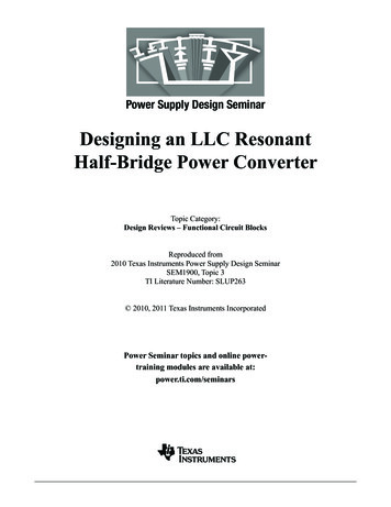
22Q e 0.1Q e 0.2Q e 0.5Q e 0.8Qe 1Qe 2Qe 5Qe 8Q e 10 2 01.61.211.61.4Q e 0.510.80.8Q e 0.10.6Q e 0.10.60.40.40.200.11.20.2Q e 0.51 Q e 10Normalized Frequency, fnQ e 0.500.1101 Q e 10Normalized Frequency, fnb. Ln 5.a. Ln 1.22Q e 0.1Q e 0.2Q e 0.5Q e 0.8Qe 1Qe 2Qe 5Qe 8Q e 10 2 0Q e 0.11.6Gain, Mg1.41.2Q e 0.5Q e 0.1Q e 0.2Q e 0.5Q e 0.8Qe 1Qe 2Qe 5Qe 8Q e 10 2 01.8Q e 0.11.61.4Gain, Mg1.810.81.21Q e 0.50.8Q e 0.1Q e 0.10.60.60.40.4Q e 0.5Q e 0.50.200.110Topic 3Gain, Mg1.4Q e 0.1Q e 0.2Q e 0.5Q e 0.8Qe 1Qe 2Qe 5Qe 8Q e 10 2 01.8Gain, Mg1.80.21 Q e 10Normalized Frequency, fn00.110c. Ln 10.1 Q e 10Normalized Frequency, fn10d. Ln 20.Fig. 6. Plots of voltage-gain function (Mg) with different values of Ln.Figs. 6a to 6d illustrate several possiblerelationships. Each plot is defined by a fixed valuefor Ln (Ln 1, 5, 10, or 20) and shows a family ofcurves with nine values, from 0.1 to 10, for thevariable Qe. From these plots, several observationscan be made.The value of Mg is not less than zero. This isobvious since Mg is from the modulus operator,which depicts a complex expression containingboth real and imaginary numbers. These numbersTexas Instrumentsrepresent both magnitude and phase angle, butonly the magnitude is useful in this case.Within a given Ln and Qe, Mg presents aconvex curve shape in the vicinity of the circuit’sresonant frequency. This is a typical curve thatshows the shape of the gain from a resonantconverter. The normalized frequency corresponding to the resonant peak (fn c0, or fsw fc0) ismoving with respect to a change in load and thusto a change in Qe for a given Ln.3-99SLUP263

Topic 3effect of Lm and shift fc0 towards f0. As a simpleillustration, it is helpful to examine two extremes:1. If RL is open, then Qe 0, and fc0 fp asdescribed by Equation (2). fc0 sits to the far leftof f0, and the corresponding gain peak is veryhigh and can be infinite in theory.2. If RL is shorted, then Qe and Lm is completely bypassed or shorted, making the effectof Lm on the gain disappear. The correspondingpeak gain value from the Lm effect thenbecomes zero, and fc0 moves all the way to theright, overlapping f0.Therefore, if RL changes from infinite to zero,the resonant peak gain changes from infinite tounity, and the corresponding frequency at peakresonance (fc0) moves from fp to the seriesresonant frequency (f0).Changing Ln and Qe will reshape the Mg curveand make it different with respect to fn. As Qe is afunction of load described by Equations (9) and(22), Mg presents a family of curves relatingfrequency modulation to variations in load.Regardless of which combination of Ln and Qeis used, all curves converge and go through thepoint of (fn, Mg) (1, 1). This point is at fn 1, orfsw f0 from Equation (20). By definition of seriesresonance, XLr – XCr 0 at f0. In other words, thevoltage drop across Lr and Cr is zero, so that theinput voltage is applied directly to the output load,resulting in a unity voltage gain of Mg 1.Notice that the operating point (fn, Mg) (1, 1)is independent of the load; i.e., as long as the gain(Mg) can be kept as unity, the switching frequencywill be at the series resonant frequency (f0) nomatter what the load current is. In other words, ina design whose operating point is at (fn, Mg) (1, 1) or its vicinity, the frequency variation isnarrowed down to minimal. At (fn, Mg) (1, 1),the impedance of the series resonant circuit iszero, assuming there are no parasitic power losses.The entire input voltage is then applied to theoutput load no matter how much the load currentvaries. However, away from (fn, Mg) (1, 1), theimpedance of the series resonant circuit becomesnonzero, the voltage gain changes with differentload impedances, and the corresponding operationbecomes load-dependent.For a fixed Ln, increasing Qe shrinks the curve,resulting in a narrower frequency-control band,which is expected since Qe is the quality factor ofthe series resonant circuit. In addition, as thewhole curve shifts lower, the corresponding peakvalue of Mg becomes smaller, and the fncorresponding to that value moves towards theright and closer to fn 1. This frequency shift withincreasing Qe is due to an increased load. It isapparent from reviewing Equations (9) and (22)that an increase in Qe may come from a reductionin RL, as both Lm and Lr are fixed. For the sameseries resonant frequency, Cr is fixed as well. RL isin parallel with Lm, so reducing RL will reduce theTexas InstrumentsFor a fixed Qe, a decrease in Ln shrinks thecurve; the whole curve is squeezed, and fc0 movestowards f0. This results in a better frequencycontrol band with a higher peak gain. There aretwo reasons for this. First, as Ln decreases due tothe decrease in Lm, fp gets closer to f0, whichsqueezes the curves from fp to f0. Second, adecreased Ln increases Lr, resulting in a higher Qe.A higher Qe shrinks the curve as just described.At first glance, it appears that any combinationof Ln and Qe would work for a converter designand that the design could be made with fn operatingon either side of fn 1. However, as explained inthe following section, there are many moreconsiderations.III. desIgn consIderAtIonsAs discussed earlier, fn is the control variablein frequency modulation. Therefore the outputvoltage can be regulated by Mg through controllingfn , as indicated by Fig. 6 and Equation (24), whichcan be rearranged as1 VVo M g (f n , L n , Qe ) in .n 23-1010(25)SLUP263

Although this discussion has so far determinedthat the design should operate in the vicinity of theseries resonance, or near fn 1, it is recommendedthat the optimum design be restricted to the areadescribed by a1 through a4 in Fig. 7, for reasons tobe explained.21.8Qe 01.6Mg max1.4Gain, MgA. What Does “In the Vicinity” Mean?a01Mg mina1Curve 1a4Cu0.6(Qe 0)rve20.4(QCuerve max)30.2Curve41fn min10fn maxNormalized Frequency, fna. In the vicinity of series resonance (near fn 1).1.6Qe 0n x Vo maxMg max Vin min /21.4a3a21.2Q e maxa01n x Vo minMg min Vin max /20.8a1a40.6Qe 01Q e maxfn minNormalized Frequency, fnfn maxb. Operation boundary set by a1 through a4.Fig. 7. Recommended design area.voltage variation over a specified range, at a givenoutput load current.Load regulation is defined as the maximumoutput-voltage variation caused by a change inload over a stated range, usually from no load tomaximum.These two types of regulation are actually achievedthrough the voltage-gain adjustment—and in anLLC converter, the gain adjustment is madethrough frequency modulation. The recommendedarea of operation described in Fig. 7 shows aFor a typical design of a power-supplyconverter, as is well-known, three basic requirements are almost always considered first—lineregulation, load regulation, and efficiency.Line regulation is defined as the maximumoutput-voltage variation caused by an input3-1111SLUP263Topic 300.1B. Basic Design RequirementsTexas Instruments1.20.8Gain, MgObviously, “in the vicinity” i

duty cycles for each switch. A small dead time is needed between the consecutive transitions, both to prevent the possibility of cross-conduction and to allow time for ZVS to be achieved. 2. The resonant circuit, also called a resonant network, consists of the resonant capacitance, Cr, and two inductances—the series resonant