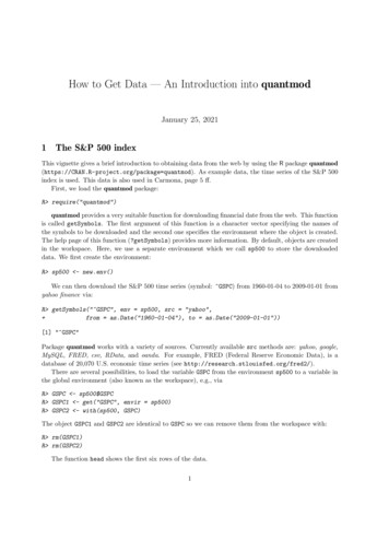
Transcription
How to Get Data — An Introduction into quantmodJanuary 25, 20211The S&P 500 indexThis vignette gives a brief introduction to obtaining data from the web by using the R package quantmod(https://CRAN.R-project.org/package quantmod). As example data, the time series of the S&P 500index is used. This data is also used in Carmona, page 5 ff.First, we load the quantmod package:R require("quantmod")quantmod provides a very suitable function for downloading financial date from the web. This functionis called getSymbols. The first argument of this function is a character vector specifying the names ofthe symbols to be downloaded and the second one specifies the environment where the object is created.The help page of this function (?getSymbols) provides more information. By default, objects are createdin the workspace. Here, we use a separate environment which we call sp500 to store the downloadeddata. We first create the environment:R sp500 - new.env()We can then download the S&P 500 time series (symbol: GSPC) from 1960-01-04 to 2009-01-01 fromyahoo finance via:R getSymbols(" GSPC", env sp500, src "yahoo", from as.Date("1960-01-04"), to as.Date("2009-01-01"))[1] " GSPC"Package quantmod works with a variety of sources. Currently available src methods are: yahoo, google,MySQL, FRED, csv, RData, and oanda. For example, FRED (Federal Reserve Economic Data), is adatabase of 20,070 U.S. economic time series (see http://research.stlouisfed.org/fred2/).There are several possibilities, to load the variable GSPC from the environment sp500 to a variable inthe global environment (also known as the workspace), e.g., viaR GSPC - sp500 GSPCR GSPC1 - get("GSPC", envir sp500)R GSPC2 - with(sp500, GSPC)The object GSPC1 and GSPC2 are identical to GSPC so we can remove them from the workspace with:R rm(GSPC1)R rm(GSPC2)The function head shows the first six rows of the data.1
R 1960-01-081960-01-11GSPC.Open GSPC.High GSPC.Low GSPC.Close GSPC.Volume 58.77This is on OHLC time series with at least the (daily) Open, Hi, Lo and Close prices for the symbol;here, it also contains the traded volume and the closing price adjusted for splits and dividends.The data object is an “extensible time series” (xts) object:R class(GSPC)[1] "xts" "zoo"Here, it is a multivariate (irregular) time series with 12334 daily observations on 6 variables:R dim(GSPC)[1] 123346Such xts objects allow for conveniently selecting single time series using R head(GSPC 0000331000032900003470000as well as very conviently selecting observations according to their time stamp by using a character “row”index in the ISO 8601 date/time format ‘CCYY-MM-DD HH:MM:SS’, where more granular elementsmay be left out in which case all observations with time stamp “matching” the given one will be used.E.g., to get all observations in March 1970:R 03-12GSPC.Open GSPC.High GSPC.Low GSPC.Close GSPC.Volume 088.332
389.63It is also possible to specify a range of timestamps using ‘/’ as the range separator, where both endpointsare optional: e.g.,R SPC.Open GSPC.High GSPC.Low GSPC.Close GSPC.Volume 000060.13gives all observations up to Epiphany (Jan 6) in 1960, andR 008-12-31GSPC.Open GSPC.High GSPC.Low GSPC.Close GSPC.Volume GSPC.Adjusted869.51873.74866.52872.80 1880050000872.80872.37873.70857.07869.42 3323430000869.42870.58891.12870.58890.64 3627800000890.64890.59910.32889.67903.25 4172940000903.25gives all observations from Christmas (Dec 25) in 2008 onwards.For OHLC time series objects, quantmod also provides convenience (column) extractors and transformers, such as Cl() for extracting the closing price, OpCl() for the transformation from opening toclosing prices, and ClCl() for the changes in closing prices:R 9.6959.5058.77R head(OpCl(GSPC))OpCl.GSPC1960-01-0403
1500GSPC1960 01 04 / 2008 12 PC.Close100010005005001e 108e 096e 094e 092e 091500GSPC.Volume1e 108e 096e 094e 092e 09GSPC.Adjusted150010001000500500Jan 041960Jan 031966Jan 031972Jan 031978Jan 031984Jan 021990Jan 021996Jan 022002Jan 022008Figure 1: Plot of GPSC via 0-01-1100000R .004305316-0.007317512-0.003183096-0.012268908One can also plot the data, either via plot() in the customary multivariate time series style:R plot(GSPC, multi.panel TRUE, yaxis.same FALSE)(see Figure 1).Alternatively, via chartSeries() in financial chart style:4
GSPC[1960 01 04/2008 12 31]Last 903.25150010005000Volume (millions):4,172,940,0001000080006000400020000Jan 04 Jan 03 Jan 03 Jan 03 Jan 03 Jan 02 Jan 02 Jan 02 Jan 02196019661972197819841990199620022008Figure 2: Plot of GSPC via chartSeries().R chartSeries(GSPC)(see Figure 2).For OHLC data, this by default gives a candlestick plot, the anatomy of which can be illustrated byzooming in:R chartSeries(GSPC["2008-12"])(see Figure 3).If we are intersted in the daily values of the weekly last-traded-day, we aggregate it by using anappropriate function from the “zoo Quick-Reference” (Shah et al., 2005). The “zoo Quick-Reference” canbe found in the web, https://CRAN.R-project.org/package zoo/vignettes/zoo-quickref.pdf, andit is strongly recommended to have a look at this vignette since it gives a very good overview of the zoopackage. Their convenience function nextfri computes for each ”Date” the next Friday.R nextfri - function(x) 7 * ceiling(as.numeric(x - 5 4)/7) as.Date(5 - 4)We get the aggregated data then viaR SP.we - aggregate(GSPC, nextfri, tail, 1)The function aggregate splits the data into subsets — here according to the function nextfri — andcomputes statistics for each, i.e., takes the last value, which is done by tail.5
[GSPC2008 12[2008 12 01/2008 12 31]920Last 903.259008808608408206000Volume (millions):4,172,940,0005000400030002000Dec 012008Dec 042008Dec 092008Dec 122008Dec 172008Dec 222008Dec 262008Dec 312008Figure 3: Plot of GSPC in Dec 2008 via chartSeries().6
This works because the data object is also a “Z’s ordered observations” (zoo) object which knows toapply nextfri() to the index (timestamps). However, this loses the xts class: if this is not desired, onecan useR SP.we - xts(aggregate(GSPC, nextfri, tail, 1))instead.Alternatively, package quantmod provides apply.weekly(), which uses a slightly different endpointstrategy:R SP.we - apply.weekly(GSPC, tail, 1)We can now extract the closing prices for the last trading day in every week:R SPC.we - Cl(SP.we)and create a plot of this time series viaR plot(SPC.we)(see Figure 4).SPC.we1960 01 08 / 2008 12 311500150010001000500500Jan 081960Jan 071966Jan 071972Jan 061978Jan 061984Jan 051990Jan 051996Jan 042002Jan 042008Figure 4: Plot of the weekly S&P 500 index closing values from 1960-01-04 to 2009-01-01.Finally, we can create log-returns “by hand” and visualize these as well7
R lr - diff(log(SPC.we))R plot(lr)(see Figure 5).lr1960 01 08 / 2008 12 310.100.100.050.050.000.00 0.05 0.05 0.10 0.10 0.15 0.15 0.20 0.20Jan 081960Jan 071966Jan 071972Jan 061978Jan 061984Jan 051990Jan 051996Jan 042002Jan 042008Figure 5: Plot of the weekly S&P 500 index log-returns values from 1960-01-04 to 2009-01-01.Alternatively, we could use periodReturn() (and relatives, specifically weeklyReturn()) from quantmod with type "log". Again, this will give slightly different values, and by default fills the leadingperiod: e.g.,R head(weeklyReturn(Cl(GSPC), type 62versusR head(lr)8
0313327690.006631425-0.009332462Investigating the NASDAQ-100 indexIn this example we want to analyze an American stock exchange, the National Association of Securities Dealers Automated Quotations, better known as NASDAQ (see http://www.nasdaq.com/ for moreinformation). It is the largest electronic screen-based equity securities trading market in the UnitedStates.Accessing x?render download allows todownload a .csv file including company symbol and name (note that there are more than 100 entries, assome companies appear with 2 symbols):R nasdaq100 read.csv("nasdaq100list.csv", stringsAsFactors FALSE, strip.white TRUE)R dim(nasdaq100)[1] 1048This has the company symbols and names in variables Symbol and Name, respectively:R names(nasdaq100)[1] "Symbol"[5] "pctchange""Name""share volume""lastsale""netchange""Nasdaq100 points" "X"R nasdaq100 Name[duplicated(nasdaq100 Name)][1] "Alphabet Inc.""Liberty Global plc"[3] "Liberty Interactive Corporation" "Twenty-First Century Fox Inc."As before we create a new environment for our NASDAQ data and use the function getSymbols ofthe quantmod package to download the NASDAQ-100 time series from 2000-01-01 to today.By using the command tryCatch we handle unusual conditions, including errors and warnings. Inthis case, if the data from a company are not available from yahoo finance, the message "Symbol .not downloadable!" is given. (For simplicity, we only download the symbols starting with ’A’.)R nasdaq - new.env()R for(i in nasdaq100 Symbol[startsWith(nasdaq100 Symbol, "A")]) { cat("Downloading time series for symbol '", i, "' .\n", sep "") status - tryCatch(getSymbols(i, env nasdaq, src "yahoo", from as.Date("2000-01-01")), error identity) if(inherits(status, "error")) cat("Symbol '", i, "' not downloadable!\n", sep "") }9
olsymbolsymbolsymbol'ATVI' .'ADBE' .'ALXN' .'ALGN' .'AMZN' .'AAL' .'AMGN' .'ADI' .'AAPL' .'AMAT' .'ASML' .'ADSK' .'ADP' .'AVGO' .E.g., the first values of the Apple time series areR with(nasdaq, 62000-01-072000-01-10AAPL.Open AAPL.High AAPL.Low AAPL.Close AAPL.Volume AAPL.Adjusted0.936384 1.004464 0.9079240.9994425357968000.8621700.966518 0.987723 0.9034600.9151795123776000.7894790.926339 0.987165 0.9196430.9285717783216000.8010330.947545 0.955357 0.8482140.8482147679728000.7317130.861607 0.901786 0.8526790.8883934607344000.7663730.910714 0.912946 0.8459820.8727685050640000.752894Further, the command chartSeries of the package quantmod provides the full financial chartingabilities to R and allows for an interaction within the charts. E.g., usingR chartSeries(nasdaq AAPL)gives a chart of the Apple values (see Figure 6) and e.g., with the command with(nasdaq,addOBV(AAPL))the On-Balance volume can be visualized in the plot. See the manual of the quantmod package (Ryan,2016) for the whole list of available plot and visualization functions.E.g., Bollinger bands consist of a center line and two price channels (bands) above and below it.The center line is an exponential moving average; the price channels are the standard deviations of thestock being studied. The bands will expand and contract as the price action of an issue becomes volatile(expansion) or becomes bound into a tight trading pattern (contraction).We can add the Bollinger Bands to a plot by using the command: addBBands(n 20, sd 2, ma "SMA", draw "bands", on -1), where n denotes the number of moving average periods, sd thenumber of standard deviations and ma the used moving average process.Have a look at the quantmod homepage for further examples and try to reproduce them, http://www.quantmod.com/examples/intro/.10
nasdaqAAPL[2000 01 03/2021 01 22]140Last 139.0700071201008060402006000Volume (millions):113,907,200400020000Jan 032000Jan 022003Jan 032006Jan 022009Jan 032012Jan 022015Figure 6: Chart of Apple.11Jan 022018Dec 312020
Jan 04 1960 Jan 03 1966 Jan 03 1972 Jan 03 1978 Jan 03 1984 Jan 02 1990 Jan 02 1996 Jan 02 2002 Jan 02 2008 GSPC 1960-01-04 / 2008-12-31 500 1000 1500 500 1000 GSPC.Open 1500 500 1000 1500 500 1000 GSPC.High 1500 500