Transcription
PROJECT SCHEDULING:IMPROVED APPROACH TO INCORPORATEUNCERTAINTY USINC BAYESIAN NETWORKSVAHID KHODAKARAMI, Queen Mary University of London, United KingdomNORMAN FENTON, Queen Mary University of London, United KingdomMARTIN NEIL, Queen Mary University of London, United KingdomIntroduction[ BSTRACf]project scheduling inevitably involvesuncertainty. The basic inputs (i.e., time,cost, and resources for each activity) arenot deterministic and are affected by various sources of uncertainty. Moreover,there is a causal relationship betweenthese uncertainty sources and projectparameters; this causality is not modeledin current state-of-the-art project planning techniques {such as simulation techniques). This paper introduces anapproach, using Bayesian network modeling, that addresses both uncertaintyand causality in project scheduling.Bayesian networks have been widely usedin a range of decision-support applications, but the application to project management is novel. The model presentedempowers the traditional critical pathmethod (CPM) to handle uncertainty andalso provides explanatory analysis to elicit, represent, and manage differentsources of uncertainty in project planning.Keywords: project scheduling;uncertainty; Bayesian networks;critical path method; CPMO1007 by the Prolett Management InstftuteVol. 3B. No. 2, 39-49, ISSN 87J6-9728/D3roject scheduling is difficult because it inevitably involves uncertainty.Uncertainty in real-world projects arises from the following characteristics;P Uniqueness (no similar experience) Variability (trade-off between performance measures like time, cost, and quality) Ambiguity (lack of clarity, lack of data, lack of structure, and bias in estimates).Matiy different techniques and tools have been developed to support betterproject scheduling, and these tools are used seriously by a large majority of project managers (Fox & Spence, 1998; Pollack-lohnson, 1998). Yet, quantifyinguncertainty is rarely prominent in these approaches.This paper focuses especially on the problem of handling uncertainty in project scheduling. The next section elaborates on the nature of uncertainty in projectscheduling and summarizes the current state of the art. The proposed approach isto adapt one of the best-used scheduling techniques, critical path method (CPM)(Kelly, 1961), and incorporate it into an explicit uncertainty model {usingBayesian networks). The paper summarizes the basic CPM methodology and notation, presents a brief introduction to Bayesian networks, and describes how theCPM approach can be incorporated (using a simple illustrative example). Also discussed is a mechanism to implement the model in real-world projects, and suggestions on how to move forward and possible future modifications are presented.The Nature of Uncertainty in Project SchedulingA Guide to the Project Management Body of Knowledge (PMBOK' Cuide)—'['hkdedi-tion (PMI, 2004) identifies risk management as a key area of project management:"Project risk management includes the processes concerned with conductingrisk management planning, identification, analysis, response, and monitoringand control on a project."Central to risk management is the issue of handling uncertainty. Ward andChapman (2003) argued that current project risk management processes induce arestricted focus on managing project uncertainty. They believe it is because theterm "risk" has become associated witb "events" rather than more general sourcesof significant uncertainty.MANAGtMENT JOLIRNM39
In different project managementprocesses there are different aspects ofuncertainty. The focus of this paper is onuncertainty in projert scheduling. Themost obvious area of uncertainty here isin estimating duration for a partiailaractivity. Difficulty in this estimation canarise from a lack of knowledge of what isinvolved as well as from the uncertainconsequences of potential threats oropportunities. This uncertainty arisesfrom one or more of the following: Level of available and requiredresources Trade-off between resources and time Possible occurrence of uncertainevents (i.e., risks) Causal factors and interdependenciesincluding common casual factorsthat affect more than one activity(such as organizational issues) Lack of previous experience and use ofsubjective rather than objective data Incomplete or imprecise data or lackof data at all Uncertainty about the basis of subjective estimation (i.e., bias in estimation).The best-known technique to support project scheduling is CPM. Thistechnique, which is adapted by themost widely used project managementsoftware tools, is purely deterministic.It makes no attempt to handle or quantify uncertainty. However, a number oftechniques, such as program evaluationand review technique (PERT), criticalchain scheduling (CCS) and MonteCarlo simulation (MCS), do try to handle uncertainty, as follows: PERT (Malcom, Roseboom, Clark, &I-azer, 1959; Miller, 1962; Moder,1988) incorporates uncertainty in arestricted sense by using a probability distribution for each task.Instead of having a single deterministic value, three different estimates(pessimistic, optimistic, and mostlikely) are approximated. Then the"critical path" and the start and finish date are calculated by the use ofdistributions' means and applyingprobability rules. Results in PERTare more realistic than CPM, butPERT does not address explicitly anyof the sources of uncertainty previously listed.40Critical chain (CC) scheduling isbased on Coldratt's theory of constraints (Coldratt, 1997). Hor minimizing the impact of Parkinson'sLaw (jobs expand to fill the allocated time), CC uses a 50% confidenceinterval for each task in projectscheduling. The safety time (remaining 50%) associated with each taskis shifted to the end of the criticalchain (longest chain) to form theproject buffer. Although it is claimedthat the CC approach is the mostimportant breakthrough in projectmanagement history, its oversimplicity is a concern for many companies that do not understand both thestrength and weakness of CC andapply it regardless of their particularand unique circumstances (Pinto,1999). The assumption that all taskdurations are overestimated by a certain factor is questionable. The mainissue is: How does the project manager determine the safety time? (Raz,Barnes, & Dvir, 2003). CC relies ona fixed, right-skewed probability foractivities, which may be inappropriate (Herroelen & Leus, 2001), and asound estimation of project andactivity duration (and consequentlythe buffer size) is still essential(Trietsch, 2005).Monte Carlo simulation (MCS) wasfirst proposed for project schedulingin the early 1960s (Van Slyke, 1963)and implemented in the 1980s(Fishman, 1986). In the 1990s,because of improvements in computer technoiogy, MCS rapidly becamethe dominant technique for handling uncertainty in project scheduling (Cook, 2001). A survey by theProject Management Institute (PMI,1999) showed that nearly 20% ofproject management software packages support MCS. For example,PertMaster(PertMaster,2006)accepts scheduling data from toolslike MS-Project and Primavera andincorporates MCS to provide projectrisk analysis in time and cost.However, the Monte Carlo approachhas attracted some criticism. VanDorp and Duffey (1999) explainedthe weakness of Monte Carlo simulation In assuming statistical inde-1007MANAGEMENT JOURNALpendence of activity duration in aproject network. Moreover, beingevent-oriented (assutning projectrisks as "independent events"),MCS and the tools that implementIt do not identify the sources ofuncertainty.As argued by Ward and Chapman(2003), managing uncertainty in projects is not just about managing perceived threats, opportunities, and theirimplication. A proper uncertaintymanagement provides for identifyingvarious sources of uncertainty, understanding the origins of them, and thenmanaging them to deal with desirableor undesirable implications.Capturing uncertainty in projects "needs to go beyond variabilityand available data. It needs toaddress ambiguity and incorporatestructure and knowledge" (Chapman& Ward, 2000). In order to measureand analyze uncertainty properly, weneed to model relations betweentrigger (source), and risk and impacts(consequences). Because projects areusually one-off experiences, theiruncertainty is epistemic (i.e., relatedto a lack of complete knowledge)rather than aleatoric (i.e., related torandomness). The duration of a taskis uncertain because there is no similar experience before, so data isincomplete and suffers from imprecision and inaccuracy. The estimationof this sort of uncertainty is mostlysubjective and based on estimatorjudgment. Any estimation is conditionally dependent on some assumptions and conditions—even ifthey are not mentioned explicitly.These assumptions and conditionsare major sources of uncertaintyand need to be addressed and handled explicitly.Themostwell-establishedapproach to handling uncertainty inthese circumstances is the Bayesianapproach (Efron, 2004; Goldstein,2006). Where complex causal relationships are involved, the Bayesianapproach is extended by usingBayesian networks. The challenge isto incorporate the CPM approachinto Bayesian networks.
The activity's "total float" (TF)(i.e., the amount that the activity'sduration can be increased withoutincreasing the overall project completion time) is the difference in the latestand earliest finish times of each activity. A critical activity is one with no TFand should receive special attention(delay in a critical activity will delaythe entire project). The critical paththen is the path(s) throiLgh the network whose activities have minimal TKCPM Methodology and NotationCPM (Moder, 1988) is a deterministictechnique that, by use of a network ofdependencies between tasks and givendeterministic values for task durations,calfulatt's the longest path in the network called the "critical path." Thelength of the "critical path" is the earliest time for project cotiipletion. Thecritical path can be identified by determining the following parameters foreach activity:The CPM approach is very simpleand provides very useful and fundamental information about a projectand its aaivities' schedule. However,because of its single-point estimateassumption, it is loo simplistic to beused in complex projects. The challenge is to incorporate the inevitableuncertainty.D—durationES—earliest start timeEF—earliest finish timeLS—latest start timeLF—latest finish time.The earliest start and finish timesof each activity are determined byworking forward through the networkand determining the earliest time atwhich an activity can start and finish,considering its predecessor activities.For each activity j\I'S, MaxjESi Di ;over predecessor activities i\EFj ESj- DjProposed BN SolutionBayesian Networks (BNs) are recognized as a mature formalism for handling causality and uncertainty(Heckerman, Mamdani, & Wellman,1995). This section provides a briefoverview of RNs and describes a newapproach for scheduling project activities in which CPM parameters (i.e., BS,EF, LS, and LF) are determined in a BN.The latest start and finish times arethe latest times that an activity canstart and finish without delaying theproject and are found by workingbackward through the network. Foreach activity i:LFj Min LFj- D,;over successor activities ;' On Time0.95Late0.05Bayesian Networks: An OverviewBayesian networks (also known asbelief networks, causal probabilisticnetworks, causal nets, graphical probability networks, probabilistic cause-Subcontracteffect tnodels, and probabilistic infiuence diagrams) provide decision support for a wide range of problemsinvolving uncertainty and probabilisticreasoning. Examples of real-worldapplications can be found inHeckerman et al. (1995), Fenton,Krause, and Neil (2002), and Neil,I enton, Forey, and I larris (2001). A BNis a directed graph, together with anassociated set of probability tables.The graph consists of nodes and arcs.Figure 1 shows a simple BN that models the cause of delay in a particulartask in a project. The nodes representuncertain variables, which may or maynot be observable. Each node has a setof states (e.g. "on time" atid "late" for"Subcontract" node). The arcs represent causal or infiuential reiationshipsbetween variables, (e.g., "subcontract"and "staff experience" may cause a"delay in task"). There is a probabilitytable for each node, providing theprobabilities of each state of the variable. For variables without parents(called "prior" nodes), the table justcontains the marginal probabilities(e.g., for the subcontract" node P(ontime) 0.95 and P(iate) 0,03). Ihis isalso caiied "prior distribution" thatrepresents the prior belief (state ofknowledge) about the variable. Foreach variable with parents, the probability table has conditional probabilities for each combination of theparents' states (see, for example, theprobability table for a "delay in task"Staff ExperienceHigh0.7Low0.3Delay in TaskSubcontractLateOn TimeStaff 0.30.99DelayFigure 1: A Bayesian network contains nodes, arcs and probability tableJUNE J007MANAUKMENT JOURNAL41
in Figure 1). This is also called the"likelihood function" that representsthe likelihood of a state of a variablegiven a particular state of its parent.The main use of BNs is in situations that require statistical inference.In addition to statements about theprobabilities of events, users havesome evidence (i.e., some variablestates or events that have actually beenobserved), and can infer the probabilities of other variables, which have notas yet been observed. These observedvalues represent a posterior probability, and by applying Bayesean rules ineach affected node, users can infiuenceother BN nodes via propagation, modifying the probability distributions. Forexample, the probability that the taskfinishes on time, with no observation,is 0.855 (see Figure 2a). However if weknow that the subcontractor failed todeliver on time, this probabilityupdates to 0.49 (see Figure 2b),BNs, as a tool for decision support,have been deployed in domains ranging from medicine to politics. BNspotentially address many of the "uncertainty" issues previously discussed. Inparticular, incorporating CPM-stylescheduling into a BN framework makesit possible to properly handle uncertainty in project scheduling.There are numerous commercialtools that enable users to build BNmodels and run the propagation calculations. With such tools it is possible toperform fast propagation in large BNs(with hundreds of nodes). In thispaper, AgenaRisk (2006) was used,since It can model continuous variables (as opposed to just discrete).BN for Activity DurationFigure 3 shows a prototype BN that theauthors have built to model uncertainty sources and their afferts on durationof a particular activity. The model contains variables that capture the uncertain nature of activity duration. "Initialduration estimation" is the first estimation of the artivity's duration; it isestimated based on historical data,previous experience, or simply expertjudgment. "Resources" incorporate anyaffeaing factor that can increase ordecrease the activity duration. It is aranked node, which for simplicity hereis restricted to three levels: low, average, and high. The level of resourcescan be inferred from so-called "indicator" nodes. Hence, the causal link isfrom the "resources" directly to observ-The key benefits of BNs that makethem highly suitable for the projectplanning domain are that they: Explicitly quantify uncertainty and modelthe causal relation between variables Enable reasoning from effert to cause aswell as from cause to effect (propagation is both "forward" and "backward") Make It possible to overturn previous beliefs in the light of new data Make predictions with incomplete data Combine subjective and objertive data Enable users to arrive at decisionsthat are based on visible auditablereasoning.Subcontractable indicator values like the "cost,"the experience of available "people"and the level of available "technology."There are many alternative indicators.An important and novel aspect of thisapproach is to allow the model to beadapted to use whichever indicatorsare available.The power of this model is betterunderstood by showing the results ofrunning it under various scenarios. It ispossible to enter observations anywhere in the model to perform not justpredictions but also many types oftrade-off and explanatory analysis. So,for example, observations for the initial duration estimation and resourcescan be entered and the model willshow the distributions for duration.Figure 4 shows how the distribution ofthe activity duration in which the initial estimation is five days changeswhen the level of its availableresources goes from low to high. (Allthe subsequent figures are outputsfrom the AgenaRisk software.)Another possible analysis in thismodel is the trade-off analysis betweenduration and resources when there is atime constraint for activity durationand it is interesting to know about thelevel of required resource. For example,consider an activity in which the initialduration is estimated as five days butmust be finished in three days. Figure 5shows the probability distribution ofrequired resources to meet this duration constraint. Note how it is skewedtoward high.Staff ExperienceStaff ExperienceDelay in TaskDelay in Task0.640.320.320.160.00.0YesNoYes(a) P(Task on fime) 0.855NoP(Task on time} 0,49Figure 2: New evidence updates the probabilityJUNH 2007PRCIIHCT M A N A I I H M E N T JOURNAI
Mapping CPM to BNThe main components of CPM networks are activities. Activities are linkedtogether to represent dependencies, lnorder to map a CPM network to a BN,it is necessary to first map a singleactivity. Each of the activity parametersare represented as a variable (node) inthe BN.Figure 6 shows a schematic modelof the BN fragment associated with anactivity. It clearly shows tbe relationbetween the activity parameters andalso the relation with predecessor andsuccessor activities.The next step is to define the connecting link between depetident activities. The forward pass in CPM ismapped as a link between the EF ofeach activity to the ES of the successoractivities. The backward-pass in CPM ismapped as a link between the LS ofeach activity to the LF of the predecessor activities.Figure 3: Bayesian network for activity durationFigure 4: Probability distribution for "duration" (days) cfianges when the level of "resources" changesLowMediumFigure 5: Level of required "Resources" when there is a constraint on "Duration"JUNK 2007HighExtwipleThe following illustrates this mappingprocess. The example is deliberatelyvery simple to avoid extra complexityin the BN. How the approach can beused in real-size projects is discussedlater in the paper.Consider a small project with fiveactivities—A, B, C, D, and E. The activity on arc (AOA) network of the projeais shown in Figure 7,The results of the CPM calculationare summarized in Table 1. ActivitiesA, C, and E with 1 F 0 are critical andthe overall project takes 20 days (i.e.,earliest finish of activity E).Figure 8 shows the full BN representation of the previous example.Each activity has five associated nodes.Forward pass calculation of CPM isdone through the connection betweenthe ES and EF. Activity A, the first activity of the project, has no predecessor,so its ES is set to zero. Activity A ispredecessor for activities B and C sothe EF of activity A is linked to the ESof activities B and C. The EF of activityB is linked to the ES of its successor,activity D. And finally, the EF of activities C and D are connected to the ES ofactivity E. In fact, the ES of activity E isthe maximum of the EF of activities CMANM FMHNT JOURN,AI.
PredecessorSuccessorActivitiesone scenario is to see how changingthe resource level affects the projectcompletion time.Figure 10 compares the distributions for project completion time asthe level of people's experiencechanges. When people's experiencechanges from low to high, the meanof finishing time changes from 22.7days to 19.5 days and the 90% confidence interval changes from 26.3days to 22.9 days.Another usefui analysis is whenthere is a constraint on tbe projectcompletion time and we want toknow how many resources are needed. Figure II illustrates this trade-offbetween project time and requiredresources. If the project needs to becompleted in 18 days (instead of thebaseline 20 days) then the resourcerequired for activity A most likelymust be high; if the project completion is set to 22, the resource level foractivity A moves significantly in thedirection of low.PredecessorActivitiesSuccessorFigure 6: Schematic of BN for an activityFigure 7: CPM networkand D. The EF of activity E is the earliest time for project completion time.The same approach is used forbackward CPM calculations connectingthe LF and LS, Activity E is the last activity of the project and has no successor,so its EF is set to EF. Activity E is successor of activities C and D so the ES ofactivity E is linked to the LF of activitiesC and D. The LS of activity D is linkedto the LF of its predecessor activity B.And finally, the LS of activities B and Care linked to the LFofactivityA. TheLFof activity A is the minimum of the LSof activities B and C.For simplicity in this example, it isassumed that activities A and E aremore risky and need more detailedanalysis. For all other activities theuncertainty about duration is expressedsimply by a normal distribution.ResultsThis section explores different scenarios of the BN model in Figure 8. Themain objective is to predict the proj-ect completion time (i.e., the earliestfinish of E) in such a way that it fullycharacterizes uncertainty.Suppose the initial estimationof activities' duration is the same asin Table 1. Suppose the resourcelevel for activities A and E is medium. If the earliest start of activity Ais set to zero, the distribution forproject completion is shown inFigure 9a. The distribution's mean is20 days as was expected from theCPM analysis. However, unlikeCPM, the prediction is not a singlepoint and Its variance is 4. Figure 9biliustrates the cumulative distribution of finishing time, which showsthe probability of completing theproject before a given time. Forexample, with a probability of 90%the project will finish in 22 days.In addition to this baseline scenario, by entering various evidence(observations) to the model, it is possible to analyze the project schedulefrom different aspects. For example.PRIMHCTJOURNALThe next scenario investigates theimpact of risk in activity A on theproject completion time as it isshown in Figure 12. When there is arisk in activity A, the mean of distribution for the project completiontime changes from 19.9 days to 22.6days and the 90% confidence intervalchanges from 22.5 days to 25.3 days.One important advantage ofBNs is their potential for parameterlearning, which is shown in thenext scenario. Imagine activity Aactually finishes in seven days,even though it was originally estimated as five days. Because activityA has taken more time than wasexpected, the level of resources hasprobably not been sufficient.By entering this observation themodel gives the resource probabilityfor activity A as illustrated in Figure13. This can update the analyst'sbelief about the actual level of available resources.Assuming both activities A and Euse the same resources (e.g., people),the updated knowledge about thelevel of available resources fromactivity A (which is finished) can beentered as evidence In the resources
DURATiONSUBNET/ i n i t i a l DuratioriNC ( Resources ( Peopie J)RiskLS AD AES AEF ALF AESLSLF BDLFDJ1 \DtJRATIONSUBNET EFigure 8: Overview of BN for example (1)for activity E (which is not startedyet) and consequently updates theproject completion time. Figure 14shows the distributions of completion time when the level of availableresource of activity E is learned fromthe actual duration of activity A.Another application of parameterlearning in these models is the abilityto incorporate and learn about bias inestimation. So, if there are severalobservations in which actual taskcompletion times are underestimated,the model learns that this may be dueJUNE 2007to bias rather than unforeseen risks,and this information will inform subsequent predictions. Work on this typeof application (caiied dynamic learnitig), is still in progress and can be apossible way of extending the BN version of CPM.P n n i t r T MANAUEMtNT JOURNAL45
113154LJJ5152015200a natural framework for abstraction andrefinement, which allows complexdomains to be described in terms ofinterrelated objects.The basic element in OOBN is anobject; an entity with an identity, state,and behavior. An object has a set ofattributes each of which is an obiect.Each object is assigned to a class.Classes provide the ability to describe ageneral, reusable network that can beused in different instances. A class inOOBN is a BN fragment.The proposed mode! has a highlyrepetitive structure and fits the objectoriented framework perfectly. Theinternal parts of the activity subnet(see Figure 6) are encapsulated withintbe activity class as shown in Figure 15.Table 1: Activities' time (days) and summary of CPM calculationsObject-Oriented BayesianNetwork (OOBN)daliy for users without much experiencein BNs. However, this complexity can behandled using the so-called object-oriented Bayesian network (OOBN)approach (Roller & Pfeffer, 1997). Thisapproach, analogous to the object-oriented programming languages, supportsII is clear from Figure 8 that even simpleCPM networks lead to fairly large BNs.In real-sized projects with several aaivities, constmaing the network needs ahuge effort, which is not effective espe-D Baseline ScenarioD Baseiine 22.024.026.010.012.014.0(a) Probability Distribution16.018.020,022.024.0(b) Cumulative DistributionFigure 9: Distribution of project completion (days) for main scenario in example (1)0.16-o- High-Quality Peopie- -o- Low-Quality People-o- High-Quality People1.0 - -o- Low-Quaiity 10.012.014.0(a) Probability16.018.020.0{b} CumulativeFigure 10: Change in project time distribution (days) when level of people's experience changesJUNE 2007 PROIECT MANAGEMENT JOURNAL22.024.026.0
Classes can be used as librariesand combined into a model as needed.By connecting interrelated objects,complex networks with several dozennodes can be constructed easily. I'igure16 shows the OOBN model for theexample previously presented.The OOBN approach can also significantly improve the performance ofinference in the model. Although a fulldiscussion of the OOBN approach tothis particular problem is beyond thescope of this paper, the key point tonote is that there is an existing mechanism (and implementation of it) thatenables the proposed solution to begenuinely "scaled-up" to real-worldprojects. Moreover, research is emerg- Complete in 18 days-o- Complete in 22 days0.480.40.320,240.160.080.0MediumLowHighFigure 1 1 : Probability of required resource changes when the time constraint changes- No Risk in A0.2 .- -o- Risk in A-a- No Risk in A1.0 n -o- Risk in A1/0,18/0.140.9IVI A/0.16\\ i\\/0.12/0.1/0.08/0.06/0.04/\\\/10.02\\10.010.0 12.0 14.0 16.0 18.0 20.0 22.0 24.0 26.010.028.012.0 14,0 16.018.0 20.0 22.0 24.026.0(b) Cumulative(a) ProbabilityFigure 12: The impact of occurring risk in activity A on the project completion timeing to develop the new generation ofBNs tools and algorithms that supportOOBN concept both in constructinglarge-scale models and also in propagation aspeas.0.8 0.72 0.64 -Conclusions and How to Move Forward0.56 -Handling risk and uncertainty isincreasingly seen as a crucial component of project management and planning. One classic problem is how toincorporate uncertainty in projectscheduling. Despite the availability ofdifferent approaches and tools, thedilemma is still challenging. Most current techniques for handling risk anduncertainty in projea scheduling (simulation-based techniques) are often0.48 0.4 0.32 0.24 0.16 -0.08 -0.0 -1LowHighMediumFigure 13: Learnt probability distribution "resource" when the actual duration is seven daysJUSiK looyPROIETTM-\NM"5FMFNT47
0.2 0.18 i- Learned Scenario- o Baseline Scenario- o Learned Scenario1.0 n -o- Baseline 028.012.014.016.0(a) Probability Graph18.020.022,024.026.0(b) Cumuiative GraphFigure 14: completion time (days) based on learned parameters compare with baseline scenarioweight and power of BN analysis tobear on the problem of project scheduling. This makes ii possible to: Capture different sources of uncertainty and use them to inform project scheduling Express uncertainty about completion time for each activity and thewhole project with full probabilitydistributions Model the trade-off between timeand resources in project activities Use "what-if?" analysis Ixarn from data so that predictionsbecome more relevant and accurate.Figure 15: Activity class encapsulates internal parts of networkBESLFLSEFt—1AESLFDESLFLSEF - EEFLF - CESLFLSLSEF)EFFigure 1 5 : 0 0 model for the presented exampleevent-oriented and try to model theimpact of possible "threats" on projectperformance. They ignore the sourceof uncertainty and the causa! relationsbetween project parameters. Moreadvanced techniques are required tocapture different aspects of uncertaintyin projects.This paper has proposed a newapproach that makes it possible to48 Iincorporate risk, uncertainty, andcausality in project scheduling.Specifically, the authors have shownhow a Bayesian network model canbe generated from a project's CPMnetwork. Part of this
dling uncertainty in project schedul-ing (Cook, 2001). A survey by the Project Management Institute (PMI, 1999) showed that nearly 20% of project management software pack-ages support MCS. For example, PertMaster (PertMaster, 2006) accepts scheduling data from tools like MS-Project and Primavera and incorporates MCS to provide project