WIXLIB

Chapter 5: Query Processing and Optimization5.15.25.35.45.55.6Evaluation of Spatial OperationsQuery OptimizationAnalysis of Spatial Index StructuresDistributed Spatial Database SystemsParallel Spatial Database SystemsSummary1

Analogy of Automatic Transmission in CarsManual transmission : automatic :: Java : SQLRecall Java program (Section 2.1.6, pp.32-34)Algorithm to answer the query was coded in the programSimilar to manual gear change at start and stop in CarsIn contrast, SQL queries are declarativeUsers do not specify the procedure to answer itDBMS needs to pick an algorithm to answer queryAnalogy: automatic transmission choosing gear (1, 2, 3, )Relevant SDBMS componentQuery processing and optimization (QPO) picks algorithms to process a SQL queryPhysical data model : QPO :: engine : automatic transmission2

What is Query Processing and Optimization (QPO)?Basic idea of QPOIn SQL, queries are expressed in high level declarative formQPO translates a SQL query to an execution plan over physical data model using operations on file-structures, indices, etc.Ideal execution plan answers Q in as little time as possibleConstraints: QPO overheads are small Computation time for QPO steps that for execution plan3

Why Learn about QPO?Why learn about automatic transmission in a car?Identify cause of lack of power in a car is it the engine or the transmission ?Solve performance problem with manual override uphill, downhill driving lower gearsWhy learn about QPO in a SDBMS?Identify performance bottleneck for a query is it the physical data model or QPO ?How to help QPO speed up processing of a query ? providing hints, rewriting query, etc.How to enhance physical data model to speed up queries? add indices, change file- structures, 4

Three Key Concepts in QPO1. Building blocksMost cars have few motions, e.g. forward, reverseSimilar most DBMS have few building blocks: select (point query, range query), join, sorting, .A SQL query is decomposed in building blocks2. Query processing strategies for building blocksCars have a few gears for forward motion: 1st, 2nd, 3rd, overdriveDBMS keeps a few processing strategies for each building block e.g. a point query can be answer via an index or via scanning data-file3. Query optimizationAutomatic transmission tries to picks best gear given motion parametersFor each building block of a given query, DBMS QPO tries to choose “most efficient” strategy given database parameters parameter examples: table size, available indices, ex. index search is chosen for a point query if the index is available5

QPO ChallengesChoice of building blocksSQL queries are based on relational algebra (RA)Building blocks of RA are select, project, join details in section 3.2 (note symbols sigma, pi and join)SQL3 adds new building blocks like transitive closure will be discussed in chapter 6Choice of processing strategies for building blocksConstraints: Too many strategies higher complexityCommercial DBMS have a total of 10 to 30 strategies 2 to 4 strategies for each building blockHow to choose the best’ strategy from among the applicable ones?May use a fixed priority schemeMay use a simple cost model based on DBMS parameters6

QPO Challenges in SDBMSBuilding Blocks for spatial queriesRich set of spatial data types, operationsA consensus on “building blocks” is lackingCurrent choices include spatial select, spatial join, nearest neighborChoice of strategiesLimited choice for some building blocks, e.g. nearest neighborChoosing best strategiesCost models are more complex since spatial queries are both CPU and I/O intensive while traditional queries are I/O intensiveCost models of spatial strategies are not mature7

QPO Challenges in SDBMS - ExerciseLearning AidOften helpful for readers to try to solve the QPO problemBefore looking at the current solutionsParticularly when solutions are not matureTry following exercise to get an insight into chapter 5 topicsExercise:Propose a few additional building blocks for spatial queries besides spatial selection, spatial join and nearest neighbor use GIS operations (Table 1.1, pp.3) as a guide if neededJustify the proposal by listing spatial queries needing the componentDetail the proposal by listing a few algorithms for the building blockHow would one choose between the available algorithms?8

Scope of DiscussionChapter 5 will discussChoice of building blocks for spatial queriesChoice of processing strategies for building blocksHow to choose the “best” strategy from among the applicable ones?Focus on concepts, not proceduresProcedures change with change in computer hardwareConcepts do not change as oftenReaders are more likely to remember the concepts after the course9

Building Blocks for Spatial QueriesChallenges in choosing building blocksRich set of data types - point, line string, polygon, Rich set of operators - topological, euclidean, set-based, Large collection of computation geometric algorithms for different spatial operations on different spatial data typesDesire to limit complexity of SDBMSHow to simplify choice of data types and operators?Reusing a Geographic Information System (GIS) which already implements spatial data types and operations however may have difficulties processing large data set on diskSDBMS reduces set of objects to be processed by a GISSDBMS is used as a filterThis is filter and refinement approach10

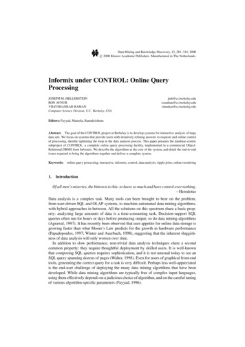
The Filter-Refine ParadigmProcessing a spatial query QFilter step : find a superset S of object in answer to Q using approximate of spatial data type and operatorRefinement step : find exact answer to Q reusing a GIS to process S using exact spatial data type and operationFilter stepRefinement stepQueryLoad object geometryTest on exactgeometrySpatial indexFigure 5.1False hitsCandidate setHitsQuery result11

Approximate Spatial Data TypesApproximating spatial data typesMinimum orthogonal bounding rectangle (MOBR or MBR) approximates line string, polygon, see examples below (black rectangle are MBRs for red objects)MBRs are used by spatial indexes, e.g. R-treeAlgorithms for spatial operations MBRs are simpleQ? Which OGIS operation (Table 3.9, pp.66) returns MBRs ?12

Approximate Spatial OperationsApproximating spatial operationsSDBMS processes MBRs for refinement stepOverlap predicate used to approximate topological operationsExample: inside(A, B) replaced by overlap(MBR(A), MBR(B)) in filter step see picture below - let A be outer polygon and B be the inner one inside(A, B) is true only if overlap(MBR(A), MBR(B)) however overlap is only a filter for inside predicate needingrefinement later13

Filter Step ExampleQuery:List objects in front of a viewer VEquivalent overlap queryDirection region is a polygonList objects overlapping with polygon( front(V))Approximate queryList objects overlapping with MBR(polygon (front (V)))14

Approximate Spatial Operations - 2Exercise: Approximate following using overlap predicateCross(A, B), Touch(A, B), Disjoint(A, B)See Table 3.9, pp.66 for definition of these operations.Exercise: Given MBRs R and S, provide conditions to testOverlap(A, B)Use coordinates of left-lower and upper-right corners of MBRs15

Choice of Building BlocksChoice of building blocksVaries across software vendors and productsRepresentative building blocks are listed hereList of building blocksPoint Query: Name a highlighted city on a digital map return one spatial object out of a tableRange Query: List all countries crossed by the river Amazon returns several objects within a spatial region from a tableSpatial Join: List all pairs of overlapping rivers and countries return pairs from 2 tables satisfying a spatial predicateNearest Neighbor: Find the city closest to Mount Everest return one spatial object from a collection16

Strategies for Each Building BlockChoice of strategiesVaries across software vendors and productsRepresentative strategies are listed hereSome strategies need special file-structures or indicesDescription of strategiesMain message: there are multiple strategies for each building block!Focus on concepts rather than proceduresReaders interested in procedural details (e.g. algorithms) refer to papers in Bibliographic notes note: better algorithms appear in literature every year!17

Strategies for Point QueriesRecall Point Query ExampleName a highlighted city on a digital mapReturn one spatial object out of a tableList of strategiesScan all B disk sectors of the data fileIf records are ordered using space filling curve (say Z-order) then use binary search on the Z-order of search point to examine about log2B disk sectorsIf an index is available on spatial location of data objects, then use find() operation on the index number of disk sector examined index depth (typically 4 to 5)18

Strategies for Range QueriesRecall Range Query ExampleList all countries crossed by of the river AmazonReturns several objects within a spatial region from a tableList of strategiesScan all B disk sectors of the data fileIf records are ordered using space filling curve (say Z-order) then determine range of Z-order values satisfying range queryuse binary search to get lowest Z-order within query answerscan forward in the data file till the highest Z-order satisfying queryIf an index is available on spatial location of data objects, then use range-query operation on the index19

Strategies for Spatial JoinsRecall Spatial Join Example:List all pairs of overlapping rivers and countries.Return pairs from 2 tables satisfying a spatial predicateList of strategiesNested loop: test all possible pairs for spatial predicate all rivers are paired with all countriesSpace Partitioning: test pairs of objects from common spatial regions only rivers in Africa are tested with countries in Africa only!Tree Matching hierarchical pairing of object groups from each tableOther, e.g. spatial-join-index based, external plane-sweep, 20

Strategies for Nearest Neighbor QueriesRecall Nearest Neighbor ExampleFind the city closest to Mount EverestReturn one spatial object from city data file CList of strategiesTwo phase approach fetch C’s disk sector(s) containing the location of Mt. Everest M minimum distance( Mt. Everest, cities in fetched sectors) test all cities within distance M of Mt. Everest (Range Query)Single phase approach recursive algorithm for R-tree eliminate candidates dominated by some other candidate21

Query Processing and Optimizer ProcessA site-seeing tripStart : a SQL QueryEnd: an execution planIntermediate Stopovers query trees logical tree transforms strategy selectionSQL GRAMMERABSTRACT DATA ISTIC URESPECIFICATIONSYSTEM CATALOGDYNAMICPROGRAMMINGWhat happens after the journey?Execution plan is executedQuery answer returnedSelectivity IndexCPUBfrCOST FUNCTIONSPATIALNONSPATIALEVALUATIONMERGEFigure 5.222

Query TreesNodes building blocks of (spatial) queriesSee section 3.2 (pp.55) for symbols sigma, pi and joinChildren inputs to a building blockLeafs TablespExample SQL query and its query tree follows:L.Names Area(L.Geometry) . 20s Fa.Name 5 ‘Campground’Distance(Fa.Geometry, L.Geometry) , 50Figure 5.3Lake LFacilities Fa23

Logical Transformation of Query Trees Motivation Transformation do not change the answer of the query But can reduce computational cost by reducing data produced by sub-queries reducing computation needs of parent node Example Transformation Push down select operation below join Example: Figure 5.4 (compare with Figure 5.3) Reduces size of table for join operations Area(L.Geometry) . 20 Other common transformations Push project down Reorder join operations .p L.NameDistance(Fa.Geometry, L.Geometry) , 50Lake LFigure 5.4s Fa.Name 5 ‘Campground’Facilities Fa24