Transcription
Layerweaver: Maximizing Resource Utilization ofNeural Processing Units via Layer-Wise SchedulingYoung H. Oh Jongsung Lee†Seonghak Kim†Yeonhong Park†Yunho Jin†Dong Uk Kim† Departmentof Electrical and Computer EngineeringSungkyunkwan University, Suwon, KoreaSam Son†Jonghyun Bae†Tae Jun Ham†Jae W. Lee†† Departmentof Computer Science and EngineeringNeural Processing Research Center (NPRC)Seoul National University, Seoul, Korea younghwan@skku.edu † ,dongukim12,taejunham,jaewlee}@snu.ac.krof tera-operations per second (TOP/s) as well as hundredsof giga-bytes per second (GB/s) DRAM bandwidth. NPUstargeting only inference tasks feature a relatively high computeto-memory bandwidth ratio (TOP/GB) [18], [20], whereas thosetargeting both inference and training a much lower ratio dueto their requirement for supporting floating-point arithmetic,which incurs larger area and bandwidth overhead.Due to a wide spectrum of arithmetic intensities of DNNmodels, there is no one-size-fit-all accelerator that works wellfor all of them. For example, convolutional neural networks(CNNs) [21]–[23] are traditionally known to be most computeintensive. In contrast, machine translation and natural languageprocessing (NLP) models [4], [24]–[26] are often composed offully-connected (FC) layers with little weight reuse to be morememory-intensive. To first order, the computational structureof a DNN model determines its arithmetic intensity, and henceits suitability to a particular NPU.Even if the arithmetic intensity of a DNN model is perfectlybalanced with the compute-to-memory ratio of the NPU, it isstill challenging to fully saturate the hardware resources. Onesuch difficulty comes from varying batch size at runtime. Forexample, the dynamic fluctuation of user requests towards aKeywords-Layer-wise Scheduling, Systems for Machine Learn- DNN serving system [13], [15], [16] or application-specifieding, Inference Serving System, Neural Networks, Accelerator batch size from cameras and sensors in an autonomous drivingSystems, Multi-taskingsystem [10], [27] mandates the system to run on a suboptimal batch size. Thus, the batch size is often highlyI. I NTRODUCTIONworkload-dependent and not freely controllable to make itWith widespread adoption of deep learning-based appli- nearly intractable to build a single NPU maintaining highcations and services, computational demands for efficient resource utilization for all such workloads.deep neural network (DNN) processing have surged in dataFor an NPU required to run diverse DNN models, a mismatchcenters [1]. In addition to already popular services such as between its compute-to-memory bandwidth ratio and theadvertisement [2], [3], social networks [4]–[7], and personal arithmetic intensity of the model being run can cause a seriousassistants [8], [9], emerging services for automobiles and IoT imbalance between compute time and memory access time.devices [10]–[12] are also attracting great attention.This yields a low system throughput due to under-utilization ofTo accelerate key deep-learning applications, datacenter either processing elements (PEs) or off-chip DRAM bandwidth,providers widely adopt high-performance serving systems [13]– which in turn translates to the cost inefficiency in datacenters.[16] based on specialized DNN accelerators, or neural process- Once either resource gets saturated (while the other resource ising units (NPUs) [17]–[19]. Such accelerators have a massive still available), it is difficult to further increase the throughputamount of computation units delivering up to several hundreds without scaling the bottlenecked resource in NPU.Abstract—To meet surging demands for deep learning inference services, many cloud computing vendors employ highperformance specialized accelerators, called neural processingunits (NPUs). One important challenge for effective use of NPUs isto achieve high resource utilization over a wide spectrum of deepneural network (DNN) models with diverse arithmetic intensities.There is often an intrinsic mismatch between the compute-tomemory bandwidth ratio of an NPU and the arithmetic intensityof the model it executes, leading to under-utilization of eithercompute resources or memory bandwidth. Ideally, we want tosaturate both compute TOP/s and DRAM bandwidth to achievehigh system throughput. Thus, we propose Layerweaver, an inference serving system with a novel multi-model time-multiplexingscheduler for NPUs. Layerweaver reduces the temporal wasteof computation resources by interweaving layer execution ofmultiple different models with opposing characteristics: computeintensive and memory-intensive. Layerweaver hides the memorytime of a memory-intensive model by overlapping it with therelatively long computation time of a compute-intensive model,thereby minimizing the idle time of the computation units waitingfor off-chip data transfers. For a two-model serving scenarioof batch 1 with 16 different pairs of compute- and memoryintensive models, Layerweaver improves the temporal utilizationof computation units and memory channels by 44.0% and 28.7%,respectively, to increase the system throughput by 60.1% onaverage, over the baseline executing one model at a time.
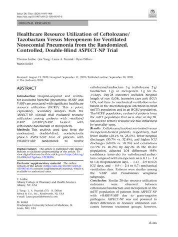
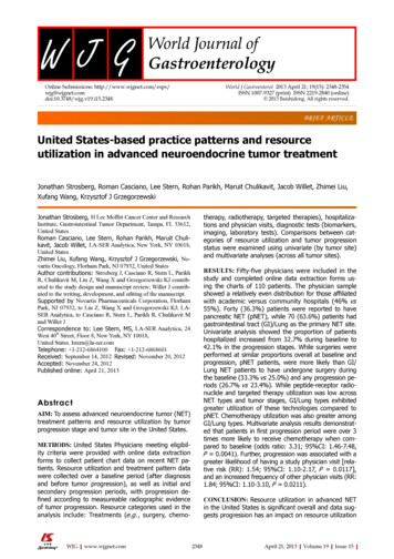
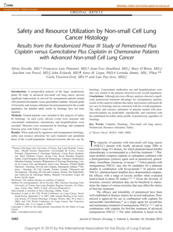
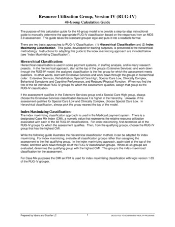
EPEArrayPE PE PE PERegisters0.00PE PE PE PEFig. 1.0.500.751.001.251.501.752.00(a) ResNeXt50 (RX)PE PE PE PEPE PE PE PEOn-chip Buffers (MB)0.25PE ArrayPEGlobal Shared BuffersOff-chip DRAMPEArrayDRAMNoC Bandwidth(GB/s)DRAMMemory Bandwidth(GB/s)0.0Compute (TOP/s)0.51.01.52.02.5(b) BERT-large (BL)Fig. 2. Layer-wise execution timeline on a unit-batch (batch 1) input inmilliseconds with (a) compute-intensive and (b) memory-intensive workload.An abstract single-chip NPU architecture.To improve resource utilization of the NPU, latency-hidingtechniques such as pipelining [28]–[30], decoupled memoryaccess and execution [31] have been proposed. These techniques overlaps compute time with memory access time byfetching dependent input activations and weights from the offchip memory while performing computation. While mitigatingthe problem to a certain extent, the imbalance between computeand memory access time eventually limits their effectiveness.To eliminate the memory bandwidth bottleneck, one popularapproach is to employ expensive high-bandwidth memorytechnologies such as HBM DRAM. However, this abundantbandwidth is wasted when running compute-intensive models(like CNNs). On the other hand, small-sized NPUs traditionallycount on double buffering [32], [33] and dataflow optimizationto minimize off-chip DRAM accesses [34]–[36].Instead, we take a software-centric approach that exploitsconcurrent execution of multiple DNN models with oppositecharacteristics to balance NPU resource utilization. To thisend, we propose Layerweaver, an inference serving systemwith a novel time-multiplexing layer-wise scheduler. Thelow-cost scheduling algorithm searches for an optimal timemultiplexed layer-wise execution order from multiple heterogeneous DNN serving requests. By interweaving the executionof both compute- and memory-intensive layers, Layerweavereffectively balances the temporal usage of both compute andmemory bandwidth resources. Our evaluation of Layerweaveron 16 pairs of compute- and memory-intensive DNN modelsdemonstrates an average of 60.1% and 53.9% improvementin system throughput for single- and multi-batch streams,respectively, over the baseline executing one model at a time.This is attributed to an increase in temporal utilization of PEsand DRAM channels by 44.0% (22.8%) and 28.7% (40.7%),respectively, for single-batch (multi-batch) streams.Our contributions are summarized as follows. We observe the existence of a significant imbalance betweenthe compute-to-memory bandwidth ratio of an NPU and thearithmetic intensity of DNN models to identify opportunities for balancing the resource usage via layer-wise timemultiplexing of multiple DNN models. We devise a novel time-multiplexing scheduler to balance theNPU resource usage, which is applicable to a wide range ofNPUs and DNN models. The proposed algorithm computes the resource idle time and selects the best schedules within acandidate group of layers. For this reason, Layerweaver findsa near-optimal schedule that achieves better performance thanheuristic approaches.We provide a detailed evaluation of Layerweaver using16 pairs of state-of-the-art DNN models with two realisticinference scenarios. We demonstrate the effectiveness ofLayerweaver for increasing system throughput by eliminatingidle cycles of compute and memory bandwidth resources.II. BACKGROUND AND M OTIVATIONA. Neural Processing UnitsWhile GPUs and FPGAs are popular for accelerating DNNworkloads, a higher efficiency can be expected by usingspecialized ASICs [17], [18], [29], [37], or neural processingunits (NPUs). Figure 1 depicts a canonical NPU architecture.A 2D array of processing elements (PE) are placed andinterconnected by a network-on-a-chip (NoC), where eachPE array has local SRAM registers. There are also globallyshared buffers to reduce off-chip DRAM accesses.Recently, with ever growing demands for energy-efficientDNN processing, specialized accelerator platforms have beenactively investigated for both datacenters [8], [20], [38], [39]and mobile/IoT devices [12], [40]–[43]. Depending on theapplication each request may be a single input instance ormini-batch with multiple instances. When a request arrivesat the host device to which an NPU is attached, it transfersmodel parameters and input data to the device-side memoryvia the PCIe interface (or on-chip bus in an SoC). Then theNPU fetches the data and commences inference computation.B. DNN Model CharacteristicsThe characteristics of a DNN is determined by the characteristics of the layers it comprises. For convolution neuralnetworks (CNNs), convolution layers typically take up themost of the inference time with the remaining time spent onbatch normalization (BN), activation, fully-connected (FC),and pooling layers. In a convolution layer most of the data(activations and filter weights) are reused with a slidingwindow, so it has a very high compute-to-memory bandwidthratio (i.e., highly compute-intensive). Figure 2(a) shows anexample execution timeline of ResNeXt50 [21], where PEs2
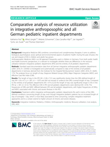
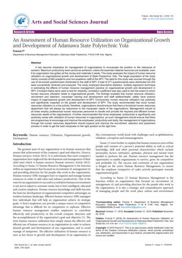
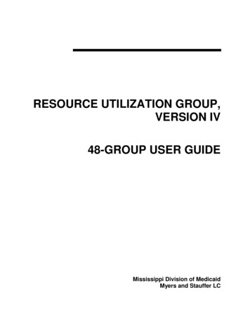
BLNCFXLICMNRNRXOP/Byte10000Active cycles (%)BBCompGoyacentricNNP-ICambriconEyeriss Mem-1000100TPUv3centric100806040200(a) Memory-centric NPUBatch 1Batch 16IC MN RN RX BB BL NCF XL IC MN RN RX BB BL NCF XLComp-intensiveMem-intensive Comp-intensiveMem-intensiveComputing utilizationMemory utilization124Batch Size8PE utilization16Active cycles (%)10100806040200Fig. 3. Compute-to-memory bandwidth ratios across varying batch sizes.Arithmetic intensity (Number of operations divided by off-chip access bytes)is measured for DNN models. Peak TOPS is divided by peak off-chip DRAMbandwidth for NPUs.are very heavily used while DRAM bandwidth is underutilized. In contrast, most neural language processing (NLP)and recommendation models are dominated by fully-connected(FC) layers which have little reuse of weight data. Thus, theFC layer has memory-intensive characteristics. As shown inFigure 2(b), BERT-large [24] has high utilization of off-chipDRAM bandwidth but much lower utilization of PEs.(b) Compute-centric NPUDRAM BW utilizationBatch 1Batch 16IC MN RN RX BB BL NCF XL IC MN RN RX BB BL NCF XLComp-intensiveMem-intensive Comp-intensiveMem-intensiveComputing utilizationMemory utilizationPE utilizationDRAM BW utilizationFig. 4. Normalized active cycles of compute-centric and memory-centricNPUs on various DNN models.Figure 4 characterizes the resource utilization in greaterdetails. The two bars for each DNN model shows normalizedactive cycles (i.e., temporal utilization) of both resources forunit-batch (batch 1) and multi-batch (batch 16) inputs, respectively. We use both compute-centric (NNP-I) and memorycentric NPUs (TPUv3) in Figure 4(a) and (b). The details ofthis experimental setup is available in Section IV-A.In Figure 4(a), the memory-centric NPU (TPUv3-like) underutilizes DRAM bandwidth for compute-intensive models andPE resources of memory-intensive models at the unit batch(batch 1, white bars). This under-utilization is explained bythe large gap between the horizontal line of the NPU and theDNN arithmetic intensity. However, at batch 16 (gray bars),memory-intensive DNN models show high PE utilization andlower DRAM bandwidth utilization compared to unit batch sizeexcept for NCF, which is extremely memory-intensive, due toan increase in the arithmetic intensity. Figure 3 shows that thepoints of the memory-intensive workloads are located abovethe horizontal line except NCF. Still, the compute-intensivemodels show very low DRAM bandwidth utilization.In Figure 4(b), the compute-centric NPU (NNP-I-like)shows opposite results. Some compute-intensive workloadsdemonstrate relatively low PE utilization because of insufficientcomputations at the unit batch. However, with batch 16, nowDRAM bandwidth is under-utilized while PE resources arefully saturated. Conversely, in the case of memory-intensiveworkloads, PE resources are still not fully saturated even atbatch 16 as DRAM bandwidth gets saturated first.C. NPU Resource Under-utilization ProblemCompute-centric vs. Memory-centric NPUs. In a datacenterenvironment NPUs are generally capable of servicing multiplerequests at once as service throughput is an important measure.In contrast, in a mobile environment, NPUs are often requiredto provide a low latency for a single request to not degrade userexperience. As such, depending on the requirements from thetarget environment, NPUs have varying compute-to-memorybandwidth ratios.Figure 3 overlays the arithmetic intensity of eight popularDNN models with the compute-to-memory bandwidth ratioof five NPUs while varying the batch size of the input. Thefollowing four of the eight models are known to be computeintensive: InceptionV3 (IC) [44], MobileNetV2 (MN) [45],ResNet50 (RN) [22] and ResNeXt50 (RX) [21]. The remainingfour models are memory-intensive: BERT-base (BB), BERTlarge (BL) [24], NCF (NCF) [26] and XLNet (XL) [25].Furthermore, we also classify five NPUs into compute-centricdesigns [18], [19], [46], which has a relatively high computeto-memory bandwidth ratio, and memory-centric designs [17],[34], which is characterized by a low ratio. If a computeintensive model (e.g., ResNeXt50) is executed on a memorycentric NPU (e.g., TPUv3), the memory bandwidth resource islikely to be under-utilized (i.e., bottlenecked by PEs) to yieldsub-optimal system throughput.Imbalance between DNN Model and NPU. There is aIII. L AYERWEAVERwide spectrum of NPUs and DNN models to make it nearlyimpossible to balance the NPU resources with the requirements A. Overviewfrom all DNN models to execute. In Figure 3, for a given NPU,The analysis in Section II-C implies that (i) either PE orthe farther the distance from the horizontal line of the NPU DRAM bandwidth resources (or both) may be under-utilizedto the arithmetic intensity of the workload, the greater degree due to a mismatch between the arithmetic intensity of a DNNof imbalance exists to yield poor resource utilization of either model and the compute-to-memory bandwidth ratio of the NPU;PEs or DRAM bandwidth. If the arithmetic intensity of the (ii) the imbalance of resource usage cannot be eliminated byDNN model in question is above the horizontal line of the simply adjusting the batch size of a single DNN model. Thus,NPU, DRAM bandwidth is under-utilized, or vice versa.we propose to execute two different DNN models with opposite3
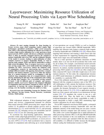
Other Workers(a)❻PEHost Processor❹ GreedySchedulerFeedbackMax windowDRAMComp. int.Model 1Model 2PE❶ LoadBalancerTimeMem. int.Request StreamsFig. 5. A timeline with different scheduling. Based on decoupled memorysystem, (a) illustrates the schedule without reordering and (b) with reordering.Fig. 6.❸❺CommandsPCIe❷ Req. QNPUNPU CoreFinish any?❼Global Buf.Interweavedµ-inst. StreamOff-chip DRAMM1C1M2C2(b)DRAM(Appended)A baseline NPU-incorporated serving system.characteristics via layer-wise time-multiplexing to balance the dequeues a certain number of requests from each queue andpass them to the scheduler. And then, 4 the host processorresource usage for a given NPU.Figure 5 illustrates how interweaving the layers of two invokes Layerweaver scheduler and performs the scheduling. 5heterogeneous DNN models can lead to balanced resource Following the scheduling result, the host processor dispatchesusage. In this setup we assume that the DNN serving system those scheduled layers to NPU by appending to activatedneeds to execute two hypothetical 3-layer models, a compute- instruction streams. 6 Depending on the scheduling results,intensive one (Model 1) and a memory-intensive one (Model 2). one of two request queues may have higher occupancy. InThe baseline schedule in Figure 5(a) does not allow reordering that case, it is reported to the cloud load balancer so that thebetween layers. During the execution of Model 2, the PE time load balancer can utilize this information for the future loadis under-utilized, whereas during the execution of Model 1, the distribution. Finally, 7 NPU executes those instructions, andDRAM time is under-utilized. However, by reordering layers once it finishes handling a single batch of requests, it returnsacross the two models appropriately as in Figure 5(b), the the result to the host processor. Note that Layerweaver employstwo models as a whole utilize both PE and DRAM bandwidth a greedy scheduler (see the next section), and thus only needsinformation about the one next layer for each model.resources in a much more balanced manner.Challenges for Efficient Layer-wise Scheduling. Determin- Baseline NPU. There exist many different types of NPUs withing an efficient schedule to fully utilize both compute and their own unique architecture. However, Layerweaver is notmemory resources is not a simple task. It would have been really dependent on the specific NPU architecture. Throughoutvery easy if the on-chip buffer had an infinite size. In such a the paper, we assume a generic NPU that resembles many ofcase, simply prioritizing layers having longer compute time the popular commercial/academic NPUs such as Google Cloudthan memory time would be sufficient to maximize compute TPUv3 [17] or Intel NNP-I [18]. This generic NPU consistsutilization as the whole memory time will be completely hidden of compute units (PEs), and two shared on-chip scratchpadby computation. However, unfortunately, the on-chip buffer memory buffers, one for weights and one for activations. Thesize is very limited, and thus one needs to carefully consider host controls this NPU by issuing a stream of commands suchthe prefetched data size as well as the remaining on-chip buffer as fetching data to on-chip memory or performing computation.size. This is because prefetching too early incurs memory idle Once the NPU finishes computation, it automatically frees thetime as described in the “Memory Idle Time” paragraph in consumed weights, and stores the outcome at the specifiedlocation of the activation buffer. One important aspect is thatSection III-D.Layerweaver. Layerweaver is an inference serving system with the NPU processes computation and main memory accessesa layer-wise weaving scheduler for NPU. The core idea of in a decoupled fashion. The NPU eagerly processes fetchLayerweaver is to interweave multiple DNN models of opposite commands from the host by performing weight transfers fromcharacteristics, thereby abating processing elements (PEs) and its main memory to the on-chip weight buffer as long as theDRAM bandwidth idle time. Figure 6 represents the overall buffer has empty space. In a similar way, its processing unitarchitecture of Layerweaver. The design goal of Layerweaver eagerly processes computation commands from the host asis to find a layer-wise schedule of execution that can finish long as its inputs (i.e., weights) are ready.all necessary computations for a given set of requests in theSupporting the layer-wise interweaving in this baselineshortest time possible.NPU does not require an extension. In fact, the NPU doesDeployment. Layerweaver is comprised of a request queue, not even need to be aware that it is running layers fromscheduler, and NPU hardware for inference computing. It different models. The host can run Layerweaver schedulercould be often integrated with a cloud load balancer that to obtain the effective layer-wise interweaved schedule, and1 directs the proper amount of inference queries for eachthen simply issue commands corresponding to the obtainedcompute- and memory-intensive models to a particular NPU schedule. Unfortunately, we find that existing commercial NPUsinstance [16], [47]–[49]. Such load-balancers are important in do not yet expose the low-level API that enables the end-userexisting systems as well since supplying an excessive number of to directly control the NPU’s scratchpad memory. However,queries to a single NPU instance can result in an unacceptable it is reasonable to assume that such APIs are internallylatency explosion. 2 Once request queues of Layerweaver available [17], [20], [50]. In this case, we believe that theaccepts the set of requests for each model, 3 the host processor developer can readily utilize Layerweaver on the target NPU.4
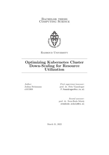
1234567891011B. Greedy Schedulerdef Schedule(MP0 , . . ., Mk 1 ):totalSteps i 0,.,k 1 (len(Mi ))curSchedule [ ]indexWindow [0, . . ., 0] # length kschedState [tm : 0, tc : 0, l :[ ]]for step in range(totalSteps):# checks for pausefor i in range(k):CheckEnd(indexWindow[i], Mi )# one scheduling stepcandidateGroup [Mi [idx] for (i, idx) inenumerate(indexWindow)]stateList [ ]for modelNum in range(k):# schedule state updatenewSchedState )stateList.append(newSchedState)# layer selectionschedState, selectedIdx Select(schedState,stateList, electedIdx])indexWindow[selectedIdx] return curScheduleThe main challenge of finding an optimal layer-wise scheduling is the enormous size of the scheduling search space. Bruteforce approach naturally leads to a burst of computation cost.For example, to find the optimal schedule for a model setconsisted of ResNet50 and BERT-base, which has 53 and 75layers respectively, 128 C53 (' 4 1036 ) candidate schedulesshould be investigated, which is not feasible. Note that theprevious work [51] uses simplified heuristics to manage the 12high search cost, while Layerweaver presents a way to formally 1314calculate the exact idle time of each resource and maximize 15the total resource utilization.To determine suitable execution order of layers for k different 1617models within a practically short time, the scheduler adopts 18a greedy layer selection approach. It estimates computationand memory idle time incurred by each candidate layer then 1920selects a layer showing the least idle time as the next scheduled 21layer. Here, the algorithm maintains a candidate group andFig. 7. Greedy layer schedule algorithm.only considers layers in the group to be scheduled next. ForS[l][0] (L3[size], t0)tmone model, a layer belongs to the group if and only if it isS[l][1] (L4[size], t1)the first unscheduled layer of the model. Assuming that anS[l][2] (L5[size], S[tc])DRAM12 3 4 5 t0 t1 tcinspection of a single potential candidate layer takes O(1) S12 3 4 5PEAlready Sched.time, the complexity for making a single scheduling decisionNewly Sched.S[l] [L3, L4, L5]is O(k). Assuming that this process is repeated for N layers,Timethe overall complexity is O(kN ) for N layers.Fig. 8. Schedule state of an example schedule S.Profiling. Before launching the scheduler, Layerweaver requires to profile a DNN model to identify computation time, It selects the layer having the shortest idle time as the nextmemory usage, and execution order of each layer. This profiling scheduled layer, which is appended to curSchedule.stage simply performs a few inference operations and thenAt the beginning of every step, CheckEnd function checksrecords information for each layer L of the model. Specifically, indexWindow[] to see if scheduling of any model is completedit records the computation time L[comp], and the number (i.e., all of its layers are scheduled). If so, the scheduler isof weights that this layer needs to fetch from the memory paused and scheduled layers up to this point (as recordedL[size]. Finally, such pairs are stored in a list M following thein curSchedule) are dispatched to NPU. Just before theoriginal execution order. Since most NPUs have a deterministic completion of execution, the scheduler is awoken and continuesperformance characteristic, offline profiling is sufficient.from where it left off. CheckEnd then probes the request queueGreedy Scheduler. Figure 7 shows the working process of in search of any remaining workload. If there is nothing left,the scheduler. We assumed NPU running Layerweaver has the scheduler is terminated. If there are additional requestsBufSize sized on-chip buffer and MemBW off-chip memory queued, they are appended to existing requests of the samebandwidth. It maintains three auxiliary data structures during model, if any. And then the scheduler resumes.its run. The algorithm selects one layer from the candidategroup and append it to the end of curSchedule every step, C. Maintaining and Updating Schedule Stateand this data structure is the outcome of Layerweaver onceThis section provides intricate detail of UpdateSchedulethe algorithm completes. indexWindow represents the indexes (Line 15 in Figure 7). The function explores the effect ofof layers in the candidate group of each model to track the scheduling a layer in the candidateGroup on the overalllayer execution progress correctly. Lastly, schedState keeps schedule and pass the information to select.several information representing the current schedule.Concept of Schedule State. Layerweaver maintains the stateFor each step the algorithm determines the next layer to for a specific schedule S. This state consists of three elebe scheduled among candidates. First, the algorithm con- ments: compute completion timestamp S[tc ], communicationstructs candidateGroup from indexWindow. Then, for each completion timestamp S[tm ], and a list S[l] containingcandidate layer UpdateSchedule function computes how the information about already scheduled layers that are expectedNPU state changes if a candidate layer is scheduled as to finish in a time interval (S[tm ], S[tc ]]. Specifically, thedescribed in Section III-C. Updated schedule states are stored list S[l] consists of pairs where each entry (S[l][j].size,in stateList. Next, Select function examines all schedule S[l][j].completion) represents the on-chip memory usagestates in stateList and estimates the idle time of each updated and the completion time of the jth layer in the list, respectively.schedule state, which will be further elaborated in Section III-D. Figure 8 illustrates an example schedule and elements com5
123456789101112131415161718Already Sched.# called by UpdateScheduledef ScheduleMemFetch(S, L):sizeToFetch L[size]PremainingBuf BufSize j S[l][j].sizecurTime S[tm ]if sizeToFetch remainingBuf:return curTime sizeToFetch / MemBWelse:curTime curTime remainingBuf / MemBWsizeToFetch - remainingBuffor j in range(len(S[l])):if curTime S[l][j].completion:curTime S[l][j].completionif sizeToFetch S[l][j].size:return curTime sizeToFetch / MemBWelse:sizeToFetch - S[l][j].sizecurTime curTime S[l][j].size / MemBWNewly Sched.S(tm)SDRAMPE12RemainingBuffer SizeMemory Idle Time/ 3S’(tm)2341423TimeFig. 10.Visualization of memory fetch scheduling.Already Sched.Fig. 9. Scheduling Memory Fetch for Layer L on Schedule S. BufSizerepresents the on-chip buffer capacity, and MemBW represents the system’smemory bandwidth.SDRAM12Compute Idle TimeNewly Sched.S(tm)S(tc)332posing its state. Below, we discuss how scheduling a specificPE1layer L changes the each element of the schedule state.S’(tm)S’(tc)Scheduling Memory Fetch. Figure 9 shows the process of1234DRAMS’(a)scheduling the memory fetch represented in pseudocode. If the1234PElayer L’s memory size L[size] is smaller than the amount ofS’(tm)available on-chip memory at time S[tm ], the memory fetch canS’(tc)234’1DRAMsimply start at S[tm ] and finish at S[tm ] L[size]/MemBW (b) S’123PE4’(Line 7). This case is shown in Figure 10(a). However, ifTimethe amount of available on-chip memory at time S[tm ] is notFig. 11. Visualization of computation scheduling.sufficient, this becomes trickier, as shown in Figure 10(b). First,a portion of L[size] that fits the currently remaining on-chip is before S’[t ] are excluded. Then, the current layer L ismmemory capacity is scheduled (Line 9). Then, the remaining appended to S[l].amount (i.e., sizeToFetch in Line 10) is scheduled when thecomputation for a layer in list S[l] completes and frees the D. Selecting a Layer to Scheduleon-chip memory. For this purpose, the code iterates over listThe goal of Layerweaver scheduler is clear: maximize bothS[l]. For each iteration, the code checks if the jth layer inthe PE utilization, and the DRAM bandwidth utilization (i.e.,the list has completed by the time that previous fetch hasbandwidth utilization of off-chip memory links). To effectivelycompleted (Line 12). If so, it immediately schedules a fetchachieve this goal, the scheduler should execute the layer thatfor the freed amount (Line 14-18). If not, it waits until thisincurs the shortest compute or memory idle time. Here, welayer completes and then schedules a fetch (Line 16-18). Thisexplain how Layerweaver estimates the amount of compute orprocess is repeated until L[size] amount of
Figure2(b), BERT-large [24] has high utilization of off-chip DRAM bandwidth but much lower utilization of PEs. C. NPU Resource Under-utilization Problem Compute-centric vs. Memory-centric NPUs. In a datacenter environment NPUs are generally capable of servicing multiple requests at once as service throughput is an important measure.