Transcription
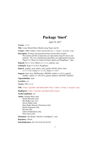
Package ‘lme4’April 19, 2017Version 1.1-13Title Linear Mixed-Effects Models using 'Eigen' and S4Contact LME4 Authors lme4-authors@lists.r-forge.r-project.org Description Fit linear and generalized linear mixed-effects models.The models and their components are represented using S4 classes andmethods. The core computational algorithms are implemented using the'Eigen' C library for numerical linear algebra and 'RcppEigen' glue''.Depends R ( 3.0.2), Matrix ( 1.1.1), methods, statsLinkingTo Rcpp ( 0.10.5), RcppEigenImports graphics, grid, splines, utils, parallel, MASS, lattice, nlme( 3.1-123), minqa ( 1.1.15), nloptr ( 1.0.4)Suggests knitr, boot, PKPDmodels, MEMSS, testthat ( 0.8.1), ggplot2,mlmRev, optimx ( 2013.8.6), gamm4, pbkrtest, HSAUR2, numDerivVignetteBuilder knitrLazyData yesLicense GPL ( 2)URL https://github.com/lme4/lme4/ http://lme4.r-forge.r-project.org/BugReports n yesAuthor Douglas Bates [aut],Martin Maechler [aut],Ben Bolker [aut, cre],Steven Walker [aut],Rune Haubo Bojesen Christensen [ctb],Henrik Singmann [ctb],Bin Dai [ctb],Gabor Grothendieck [ctb],Peter Green [ctb]Maintainer Ben Bolker bbolker lme4@gmail.com Repository CRANDate/Publication 2017-04-19 04:28:18 UTC1
R topics documented:2R topics documented:lme4-package . . . .Arabidopsis . . . . .bootMer . . . . . . .cake . . . . . . . . .cbpp . . . . . . . . .checkConv . . . . .confint.merMod . . .convergence . . . . .devcomp . . . . . . .drop1.merMod . . .dummy . . . . . . .Dyestuff . . . . . . .expandDoubleVerts .factorize . . . . . . .findbars . . . . . . .fixef . . . . . . . . .fortify . . . . . . . .getME . . . . . . . .GHrule . . . . . . .glmer . . . . . . . .glmer.nb . . . . . . .glmerLaplaceHandleglmFamily . . . . . .glmFamily-class . . .golden-class . . . . .GQdk . . . . . . . .grouseticks . . . . .hatvalues.merMod . .InstEval . . . . . . .isNested . . . . . . .isREML . . . . . . .lmer . . . . . . . . .lmerControl . . . . .lmList . . . . . . . .lmList4-class . . . .lmResp . . . . . . .lmResp-class . . . .merMod-class . . . .merPredD . . . . . .merPredD-class . . .mkdevfun . . . . . .mkMerMod . . . . .mkRespMod . . . . .mkReTrms . . . . .mkSimulateTemplatemkVarCorr . . . . 738394040414450515253545859606161626364
lme4-packagemodular . . . . .NelderMead . . .NelderMead-classngrps . . . . . .nlformula . . . .nlmer . . . . . .nloptwrap . . . .nobars . . . . . .Pastes . . . . . .Penicillin . . . .plot.lmList4 . . .plot.merMod . .plots.thpr . . . .predict.merMod .profile-methods .prt-utilities . . . .pvalues . . . . .ranef . . . . . . .refit . . . . . . .refitML . . . . .rePos . . . . . .rePos-class . . .residuals.merModsigma . . . . . .simulate.merModsleepstudy . . . .subbars . . . . .troubleshooting .VarCorr . . . . .vcconv . . . . . .VerbAgg . . . . , generalized linear, and nonlinear mixed modelsDescriptionlme4 provides functions for fitting and analyzing mixed models: linear (lmer), generalized linear(glmer) and nonlinear (nlmer.)
4lme4-packageDifferences between nlme and lme4lme4 covers approximately the same ground as the earlier nlme package. The most importantdifferences are: lme4 uses modern, efficient linear algebra methods as implemented in the Eigen package, anduses reference classes to avoid undue copying of large objects; it is therefore likely to be fasterand more memory-efficient than nlme. lme4 includes generalized linear mixed model (GLMM) capabilities, via the glmer function. lme4 does not currently implement nlme’s features for modeling heteroscedasticity and correlation of residuals. lme4 does not currently offer the same flexibility as nlme for composing complex variancecovariance structures, but it does implement crossed random effects in a way that is both easierfor the user and much faster. lme4 offers built-in facilities for likelihood profiling and parametric bootstrapping. lme4 is designed to be more modular than nlme, making it easier for downstream packagedevelopers and end-users to re-use its components for extensions of the basic mixed modelframework. It also allows more flexibility for specifying different functions for optimizingover the random-effects variance-covariance parameters. lme4 is not (yet) as well-documented as nlme.Differences between current (1.0. ) and previous versions of lme4 [gn]lmer now produces objects of class merMod rather than class mer as before the new version uses a combination of S3 and reference classes (see ReferenceClasses,merPredD-class, and lmResp-class) as well as S4 classes; partly for this reason it is moreinteroperable with nlme The internal structure of [gn]lmer is now more modular, allowing finer control of the differentsteps of argument checking; construction of design matrices and data structures; parameterestimation; and construction of the final merMod object (see modular) profiling and parametric bootstrapping are new in the current version the new version of lme4 does not provide an mcmcsamp (post-hoc MCMC sampling) method,because this was deemed to be unreliable. Alternatives for computing p-values include parametric bootstrapping (bootMer) or methods implemented in the pbkrtest package and leveraged by the lmerTest package and the Anova function in the car package (see pvalues formore details).Caveats and trouble-shooting Some users who have previously installed versions of the RcppEigen and minqa packages mayencounter segmentation faults (!!); the solution is to make sure to re-install these packagesbefore installing lme4. (Because the problem is not with the explicit version of the packages,but with running packages that were built with different versions of Rcpp in conjunction witheach other, simply making sure you have the latest version, or using update.packages, willnot necessarily solve the problem; you must actually re-install the packages. The problem ismost likely with minqa.)
ArabidopsisArabidopsis5Arabidopsis clipping/fertilization dataDescriptionData on genetic variation in responses to fertilization and simulated herbivory in ArabidopsisUsagedata("Arabidopsis")FormatA data frame with 625 observations on the following 8 variables.reg region: a factor with 3 levels NL (Netherlands), SP (Spain), SW (Sweden)popu population: a factor with the form n.R representing a population in region Rgen genotype: a factor with 24 (numeric-valued) levelsrack a nuisance factor with 2 levels, one for each of two greenhouse racksnutrient fertilization treatment/nutrient level (1, minimal nutrients or 8, added nutrients)amd simulated herbivory or "clipping" (apical meristem damage): unclipped (baseline) or clippedstatus a nuisance factor for germination method (Normal, Petri.Plate, or Transplant)total.fruits total fruit set per plant (integer)SourceFrom Josh BantaReferencesJoshua A. Banta, Martin H. H Stevens, and Massimo Pigliucci (2010) A comprehensive test of the’limiting resources’ framework applied to plant tolerance to apical meristem damage. Oikos 119(2),359–369; .fruits 1) amd nutrient, data Arabidopsis,groups gen,strip strip.custom(strip.names c(TRUE,TRUE)),type c('p','a'), ## points and panel-average value -## see ?panel.xyplotscales list(x list(rot 90)),main "Panel: nutrient, Color: genotype")
6bootMerbootMerModel-based (Semi-)Parametric Bootstrap for Mixed ModelsDescriptionPerform model-based (Semi-)parametric bootstrap for mixed models.UsagebootMer(x, FUN, nsim 1, seed NULL, use.u FALSE, re.form NA,type c("parametric", "semiparametric"),verbose FALSE, .progress "none", PBargs list(),parallel c("no", "multicore", "snow"),ncpus getOption("boot.ncpus", 1L), cl NULL)Argumentsxa fitted merMod object: see lmer, glmer, etc.FUNa function taking a fitted merMod object as input and returning the statistic ofinterest, which must be a (possibly named) numeric vector.nsimnumber of simulations, positive integer; the bootstrap B (or R).seedoptional argument to set.seed.use.ulogical, indicating whether the spherical random effects should be simulated /bootstrapped as well. If TRUE, they are not changed, and all inference is conditional on these values. If FALSE, new normal deviates are drawn (see Details).re.formformula, NA (equivalent to use.u FALSE), or NULL (equivalent to use.u TRUE):alternative to use.u for specifying which random effects to incorporate. Seesimulate.merMod for details.typecharacter string specifying the type of bootstrap, "parametric" or "semiparametric";partial matching is allowed.verboselogical indicating if progress should print output.progresscharacter string - type of progress bar to display. Default is "none"; the functionwill look for a relevant *ProgressBar function, so "txt" will work in general;"tk" is available if the tcltk package is loaded; or "win" on Windows systems.Progress bars are disabled (with a message) for parallel operation.PBargsa list of additional arguments to the progress bar function (the package authorslike list(style 3)).parallelThe type of parallel operation to be used (if any). If missing, the default is takenfrom the option "boot.parallel" (and if that is not set, "no").ncpusinteger: number of processes to be used in parallel operation: typically onewould choose this to be the number of available CPUs.clAn optional parallel or snow cluster for use if parallel "snow". If notsupplied, a cluster on the local machine is created for the duration of the bootcall.
bootMer7DetailsThe semi-parametric variant is only partially implemented, and we only provide a method for lmerand glmer results.The working name for bootMer() was “simulestimate()”, as it is an extension of simulate (seesimulate.merMod), but we want to emphasize its potential for valid inference. If use.u is FALSE and type is "parametric", each simulation generates new values of boththe “spherical” random effects u and the i.i.d. errors , using rnorm() with parameters corresponding to the fitted model x. If use.u is TRUE and type "parametric", only the i.i.d. errors (or, for GLMMs, responsevalues drawn from the appropriate distributions) are resampled, with the values of u stayingfixed at their estimated values. If use.u is TRUE and type "semiparametric", the i.i.d. errors are sampled from the distribution of (response) residuals. (For GLMMs, the resulting sample will no longer have thesame properties as the original sample, and the method may not make sense; a warning isgenerated.) The semiparametric bootstrap is currently an experimental feature, and thereforemay not be stable. The case where use.u is FALSE and type "semiparametric" is not implemented; Morris(2002) suggests that resampling from the estimated values of u is not good practice.Valuean object of S3 class "boot", compatible with boot package’s boot() result.ReferencesDavison, A.C. and Hinkley, D.V. (1997) Bootstrap Methods and Their Application. CambridgeUniversity Press.Morris, J. S. (2002). The BLUPs Are Not ‘best’ When It Comes to Bootstrapping. Statistics &Probability Letters 56(4): 425–430. doi:10.1016/S0167-7152(02)00041-X.See Also confint.merMod, for a more specific approach to bootstrap confidence intervals on parameters. refit(), or PBmodcomp() from the pbkrtest package, for parametric bootstrap comparisonof models. boot(), and then boot.ci, from the boot package. profile-methods, for likelihood-based inference, including confidence intervals. pvalues, for more general approaches to inference and p-value computation in mixed models.Examplesfm01ML - lmer(Yield 1 Batch, Dyestuff, REML FALSE)## see ?"profile-methods"mySumm - function(.) { s - sigma(.)c(beta getME(., "beta"), sigma s, sig01 unname(s * getME(., "theta"))) }
8bootMer(t0 - mySumm(fm01ML)) # just three parameters## alternatively:mySumm2 - function(.) {c(beta fixef(.),sigma sigma(.), sig01 sqrt(unlist(VarCorr(.))))}set.seed(101)## 3.8s (on a 5600 MIPS 64bit fast(year 2009) desktop "AMD Phenom(tm) II X4 925"):system.time( boo01 - bootMer(fm01ML, mySumm, nsim 100) )## to "look" at itrequire("boot") ## a recommended package, i.e. *must* be thereboo01## note large estimated bias for sig01## ( 30% low, decreases slightly for nsim 1000)## extract the bootstrapped values as a data frame .head(as.data.frame(boo01))## ------ Bootstrap-based confidence intervals -----------## warnings about "Some . intervals may be unstable" go away##for larger bootstrap samples, e.g. nsim 500## intercept(bCI.1 - boot.ci(boo01, index 1, type c("norm", "basic", "perc")))# beta## Residual standard deviation - original scale:(bCI.2 - boot.ci(boo01, index 2, type c("norm", "basic", "perc")))## Residual SD - transform to log scale:(bCI.2L - boot.ci(boo01, index 2, type c("norm", "basic", "perc"),h log, hdot function(.) 1/., hinv exp))## Among-batch variance:(bCI.3 - boot.ci(boo01, index 3, type c("norm", "basic", "perc"))) # sig01## Copy of unexported stats:::format.perc helper functionformat.perc - function(probs, digits) {paste(format(100 * probs, trim TRUE,scientific FALSE, digits digits),"%")}## Extract all CIs (somewhat awkward)bCI.tab - function(b,ind length(b t0), type "perc", conf 0.95) {btab0 - dex i,conf conf, type type) percent))btab - btab0[,4:5]rownames(btab) - names(b t0)a - (1 - conf)/2a - c(a, 1 - a)
cake9pct - format.perc(a, 3)colnames(btab) - pctreturn(btab)}bCI.tab(boo01)## Graphical examination:plot(boo01,index 3)## Check stored values from a longer (1000-replicate) run:(load(system.file("testdata","boo01L.RData", package "lme4")))# "boo01L"plot(boo01L, index 3)mean(boo01L t[,"sig01"] 0) ## note point mass at zero!cakeBreakage Angle of Chocolate CakesDescriptionData on the breakage angle of chocolate cakes made with three different recipes and baked at sixdifferent temperatures. This is a split-plot design with the recipes being whole-units and the different temperatures being applied to sub-units (within replicates). The experimental notes suggest thatthe replicate numbering represents temporal ordering.FormatA data frame with 270 observations on the following 5 variables.replicate a factor with levels 1 to 15recipe a factor with levels A, B and Ctemperature an ordered factor with levels 175 185 195 205 215 225angle a numeric vector giving the angle at which the cake broke.temp numeric value of the baking temperature (degrees F).DetailsThe replicate factor is nested within the recipe factor, and temperature is nested within replicate.SourceOriginal data were presented in Cook (1938), and reported in Cochran and Cox (1957, p. 300).Also cited in Lee, Nelder and Pawitan (2006).
10cbppReferencesCook, F. E. (1938) Chocolate cake, I. Optimum baking temperature. Master’s Thesis, Iowa StateCollege.Cochran, W. G., and Cox, G. M. (1957) Experimental designs, 2nd Ed. New York, John Wiley \&Sons.Lee, Y., Nelder, J. A., and Pawitan, Y. (2006) Generalized linear models with random effects.Unified analysis via H-likelihood. Boca Raton, Chapman and Hall/CRC.Examplesstr(cake)## 'temp' is continuous, 'temperature' an ordered factor with 6 levels(fm1 - lmer(angle recipe * temperature (1 recipe:replicate), cake, REML FALSE))(fm2 - lmer(angle recipe temperature (1 recipe:replicate), cake, REML FALSE))(fm3 - lmer(angle recipe temp (1 recipe:replicate), cake, REML FALSE))## and now "choose" :anova(fm3, fm2, fm1)cbppContagious bovine pleuropneumoniaDescriptionContagious bovine pleuropneumonia (CBPP) is a major disease of cattle in Africa, caused by amycoplasma. This dataset describes the serological incidence of CBPP in zebu cattle during afollow-up survey implemented in 15 commercial herds located in the Boji district of Ethiopia. Thegoal of the survey was to study the within-herd spread of CBPP in newly infected herds. Bloodsamples were quarterly collected from all animals of these herds to determine their CBPP status.These data were used to compute the serological incidence of CBPP (new cases occurring during agiven time period). Some data are missing (lost to follow-up).FormatA data frame with 56 observations on the following 4 variables.herd A factor identifying the herd (1 to 15).incidence The number of new serological cases for a given herd and time period.size A numeric vector describing herd size at the beginning of a given time period.period A factor with levels 1 to 4.DetailsSerological status was determined using a competitive enzyme-linked immuno-sorbent assay (cELISA).
checkConv11SourceLesnoff, M., Laval, G., Bonnet, P., Abdicho, S., Workalemahu, A., Kifle, D., Peyraud, A., Lancelot,R., Thiaucourt, F. (2004) Within-herd spread of contagious bovine pleuropneumonia in Ethiopianhighlands. Preventive Veterinary Medicine 64, 27–40.Examples## response as a matrix(m1 - glmer(cbind(incidence, size - incidence) period (1 herd),family binomial, data cbpp))## response as a vector of probabilities and usage of argument "weights"m1p - glmer(incidence / size period (1 herd), weights size,family binomial, data cbpp)## Confirm that these are equivalent:stopifnot(all.equal(fixef(m1), fixef(m1p), tolerance 1e-5),all.equal(ranef(m1), ranef(m1p), tolerance 1e-5))## GLMM with individual-level variability (accounting for overdispersion)cbpp obs - 1:nrow(cbpp)(m2 - glmer(cbind(incidence, size - incidence) period (1 herd) (1 obs),family binomial, data cbpp))checkConvExtended Convergence CheckingDescriptionPrimarily internal code for checking optimization convergence, see convergence for a more detaileddiscussion.UsagecheckConv(derivs, coefs, ctrl, lbound, debug FALSE)Argumentsderivstypically the "derivs" attribute of optimizeLmer(); with "gradients" and possibly "Hessian" componentcoefscurrent coefficient estimatesctrllist of lists, each with action character strings specifying what should happen when a check triggers, and tol numerical tolerances, as is the result oflmerControl() checkConv.lboundvector of lower bounds for random-effects parameters only (length is taken todetermine number of RE parameters)debugenable debugging output, useful if some checks are on "ignore", but would "trigger"
12confint.merModValueA result list containingcodeThe return code for the checkmessagesA character vector of warnings and messages generated by the checkSee Alsoconvergenceconfint.merModCompute Confidence Intervals for Parameters of a [ng]lmer FitDescriptionCompute confidence intervals on the parameters of a *lmer() model fit (of class"merMod").Usage## S3 method for class 'merMod'confint(object, parm, level 0.95,method c("profile", "Wald", "boot"), zeta,nsim 500,boot.type c("perc","basic","norm"),FUN NULL, quiet FALSE,oldNames TRUE, .)Argumentsobjecta fitted [ng]lmer modelparmparameters for which intervals are sought. Specified by an integer vector ofpositions, character vector of parameter names, or (unless doing parametricbootstrapping with a user-specified bootstrap function) "theta " or "beta "to specify variance-covariance or fixed effects parameters only: see the whichparameter of profile.levelconfidence level 1, typically above 0.90.methoda character string determining the method for computing the confidence intervals.zeta(for method "profile" only:) likelihood cutoff (if not specified, as by default, computed from level).nsimnumber of simulations for parametric bootstrap intervals.FUNbootstrap function; if NULL, an internal function that returns the fixed-effect parameters as well as the random-effect parameters on the standard deviation/correlationscale will be used. See bootMer for details.
confint.merMod13boot.typebootstrap confidence interval type, as described in boot.ci. (Methods ‘stud’and ‘bca’ are unavailable because they require additional components to be calculated.)quiet(logical) suppress messages about computationally intensive profiling?oldNames(logical) use old-style names for variance-covariance parameters, e.g. ".sig01",rather than newer (more informative) names such as "sd (Intercept) Subject"?(See signames argument to profile).additional parameters to be passed to profile.merMod or bootMer, respectively.DetailsDepending on the method specified, confint() computes confidence intervals by"profile": computing a likelihood profile and finding the appropriate cutoffs based on the likelihood ratio test;"Wald": approximating the confidence intervals (of fixed-effect parameters only; all variancecovariance parameters CIs will be returned as NA) based on the estimated local curvature ofthe likelihood surface;"boot": performing parametric bootstrapping with confidence intervals computed from the bootstrap distribution according to boot.type (see bootMer, boot.ci).Valuea numeric table (matrix with column and row names) of confidence intervals; the confidence intervals are computed on the standard deviation scale.NoteThe default method "profile" amounts toconfint(profile(object, which parm), signames oldNames, .),level, zeta)where the profile method profile.merMod does almost all the computations. Therefore it istypically advisable to store the profile(.) result, say in pp, and then use confint(pp, level *)e.g., for different levels.Examplesfm1 - lmer(Reaction Days (Days Subject), sleepstudy)fm1W - confint(fm1, method "Wald")# very fast, but .fm1WtestLevel - if (nzchar(s - Sys.getenv("LME4 TEST LEVEL"))) as.numeric(s) else 1if(interactive() testLevel 3) {## 20 seconds, MacBook Pro laptopsystem.time(fm1P - confint(fm1, method "profile", ## defaultoldNames FALSE))## 40 seconds
14convergencesystem.time(fm1B - confint(fm1,method "boot",.progress "txt", PBargs list(style 3)))} elseload(system.file("testdata","confint ex.rda",package "lme4"))fm1Pfm1BconvergenceAssessing Convergence for Fitted ModelsDescriptionThe lme4 package uses general-purpose nonlinear optimizers (e.g. Nelder-Mead or Powell’s BOBYQAmethod) to estimate the variance-covariance matrices of the random effects. Assessing reliablywhether such algorithms have converged is difficult. For example, evaluating the Karush-KuhnTucker conditions (convergence criteria which in the simplest case of non-constrained optimizationreduce to showing that the gradient is zero and the Hessian is positive definite) is challenging because of the difficulty of evaluating the gradient and Hessian.We (the lme4 authors and maintainers) are still in the process of finding the best strategies for testingconvergence. Some of the relevant issues are the gradient and Hessian are the basic ingredients of KKT-style testing, but when they haveto be estimated by finite differences (as in the case of lme4; direct computation of derivativesbased on analytic expressions may eventually be available for some special classes, but wehave not yet implemented them) they may not be sufficiently accurate for reliable convergencetesting. The Hessian computation in particular represents a difficult tradeoff between computationalexpense and accuracy. At present the Hessian computations used for convergence checking(and for estimating standard errors of fixed-effect parameters for GLMMs) follow the ordinalpackage in using a naive but computationally cheap centered finite difference computation(with a fixed step size of 10 4 ). A more reliable but more expensive approach is to useRichardson extrapolation, as implemented in the numDeriv package. it is important to scale the estimated gradient at the estimate appropriately; two reasonableapproaches are1. don’t scale random-effects (Cholesky) gradients, since these are essentially already unitless (for LMMs they are scaled relative to the residual variance; for GLMMs they arescaled relative to the sampling variance of the conditional distribution); for GLMMs,scale fixed-effect gradients by the standard deviations of the corresponding input variable, or2. scale gradients by the inverse Cholesky factor of the Hessian, equivalent to scaling bythe estimated Wald standard error of the estimated parameters. The latter approach isused in the current version of lme4; it has the disadvantage that it requires us to estimatethe Hessian (although the Hessian is required for reliable estimation of the fixed-effectstandard errors for GLMMs in any case).
convergence15 Exploratory analyses suggest that (1) the naive estimation of the Hessian may fail for largedata sets (number of observations greater than approximately 105 ); (2) the magnitude of thescaled gradient increases with sample size, so that warnings will occur even for apparentlywell-behaved fits with large data sets.If you do see convergence warnings, and want to trouble-shoot/double-check the results, the following steps are recommended (examples are given below): double-check the model specification and the data for mistakes center and scale continuous predictor variables (e.g. with scale) check for singularity: if any of the diagonal elements of the Cholesky factor are zero or verysmall, the convergence testing methods may be inappropriate (see examples) double-check the Hessian calculation with the more expensive Richardson extrapolation method(see examples) restart the fit from the apparent optimum, or from a point perturbed slightly away from theoptimum try all available optimizers (e.g. several different implementations of BOBYQA and NelderMead, L-BFGS-B from optim, nlminb, . . . ) While this will of course be slow for largefits, we consider it the gold standard; if all optimizers converge to values that are practicallyequivalent, then we would consider the convergence warnings to be false positives.To quote Douglas Adams, we apologize for the inconvenience.See AlsolmerControlExamplesfm1 - lmer(Reaction Days (Days Subject), sleepstudy)## 1. center and scale predictors:ss.CS - transform(sleepstudy, Days scale(Days))fm1.CS - update(fm1, data ss.CS)## 2. check singularitydiag.vals - getME(fm1,"theta")[getME(fm1,"lower") 0]any(diag.vals 1e-6) # FALSE## 3. recompute gradient and Hessian with Richardson extrapolationdevfun - update(fm1, devFunOnly TRUE)if (isLMM(fm1)) {pars - getME(fm1,"theta")} else {## GLMM: requires both random and fixed parameterspars - getME(fm1, c("theta","fixef"))}if (require("numDeriv")) {cat("hess:\n"); print(hess - hessian(devfun, unlist(pars)))cat("grad:\n"); print(grad - grad(devfun, unlist(pars)))
16devcompcat("scaled gradient:\n")print(scgrad - solve(chol(hess), grad))}## compare with internal calculations:fm1@optinfo derivs## 4. restart the fit from the original value (or## a slightly perturbed value):fm1.restart - update(fm1, start pars)## 5. try all available optimizerssource(system.file("utils", "allFit.R", package "lme4"))fm1.all - allFit(fm1)ss - summary(fm1.all)ss fixef#
April 19, 2017 Version 1.1-13 Title Linear Mixed-Effects Models using 'Eigen' and S4 Contact LME4 Authors lme4-authors@lists.r-forge.r-project.org Description Fit linear and generalized linear mixed-effects models. The models and their components are represented using S4 classes and methods. The core computational algorithms are implemented .
