Transcription
SFB 6 4 9Rainer Schulz*Martin Wersing*Axel Werwatz**ECONOMIC RISKAutomated ValuationModelling:A SpecificationExerciseBERLINSFB 649 Discussion Paper 2013-046*University of Aberdeen Business School, United Kingdom**Technische Universität Berlin, GermanyThis research was supported by the DeutscheForschungsgemeinschaft through the SFB 649 "Economic Risk".http://sfb649.wiwi.hu-berlin.deISSN 1860-5664SFB 649, Humboldt-Universität zu BerlinSpandauer Straße 1, D-10178 Berlin
Automated Valuation Modelling: A Specification ExerciseRainer Schulz, Martin Wersing, and Axel Werwatz September 2013 Schulz and Wersing: University of Aberdeen Business School, Edward Wright Building, Dunbar Street, Aberdeen AB24 3QY, United Kingdom.Emails: r.schulz@abdn.ac.uk and martin.wersing@abdn.ac.uk. Werwatz: Technische Universität Berlin, Institut für Volkswirtschaftslehreund Wirtschaftsrecht, Straße des 17. Juni 135, 10623 Berlin, Germany, and Collaborative ResearchCenter 649 Economic Risk, Humboldt-Universität zu Berlin. Email: axel.werwatz@tu-berlin.de.1
AbstractMarket value predictions for residential properties are important for investmentdecisions and the risk management of households, banks, and real estate developers.The increased access to market data has spurred the development and applicationof Automated Valuation Models (AVMs), which can provide appraisals at low cost.We discuss the stages involved when developing an AVM. By reflecting on our experience with md*immo, an AVM from Berlin, Germany, our paper contributes toan area that has not received much attention in the academic literature. In addition to discussing the main stages of AVM development, we examine empiricallythe statistical model development and validation step. We find that automatedoutlier removal is important and that a log model performs best, but only if itaccounts for the retransformation problem and heteroscedasticity.Keywords: Hedonic regression, log transformation, predictive performance2
1IntroductionThe market value of a residential property is the price one should expect in an arm’slength transaction between informed and willing buyers and sellers. This value dependson the property’s structural and location characteristics, some of these can be observedeasily, but others will require a full physical inspection. Professional valuers predictthe market value of a property by taking all characteristics into account. Such afull appraisal should provide an accurate prediction of the market value, but is alsotime consuming and expensive. Automated Valuation Models (AVMs) use recordedtransaction or listing information to fit a statistical model. Once the model is fitted,the market value of any common type of residential property can be predicted. Suchautomated appraisals might be less accurate than full appraisals, but are also less costly.Market participants will be prepared to trade off predictive accuracy for cost inseveral applications. First, banks can use low cost appraisals from AVM services whenunderwriting further loan advances, home equity withdrawals, and remortgaging (FitchRatings Structured Finance, 2012). Bank risk managers may use an AVM as a costeffective tool to monitor the collateral values underlying the bank’s portfolio of mortgage loans. Such monitoring can be required by banking regulation. Second, AVMappraisals are also used when mortgage loans are pooled and securitised. Rating agencies request information about current loan-to-value ratios, as they relate to defaultprobabilities and loss severity given default, and AVM appraisals contribute to suchinformation (Moody’s Investors Service, 2009, 2012). Third, aspiring property ownersmight want to get a feel for the expected price they have to pay for their dream house.Existing property owners might be interested in a snapshot appraisal, maybe to informthe decision to relocate. An appraisal from an AVM service will fit the bill. The availability of low cost appraisals should, therefore, increase the transparency of residentialproperty markets. Fourth, government agencies might be interested in cost-effectiveappraisals for taxation, planning, and land use regulation (IAAO, 2003).In Europe, several providers offer AVM services. Examples are Calnea, Hometrack,and RightmoveData in the UK, Calcasa in the Netherlands, and ImmobilienScout24and md*immo in Germany. As most of these services are proprietary businesses, onlylimited information can be obtained about how a specific AVM is implemented. Atthe same time, there is no scarcity of academic papers examining house prices with3
statistical models. This literature mostly focusses on the construction of house priceindices or the estimation of marginal valuations of individual property characteristics(Hill et al., 1997; Palmquist, 1980, 1991). Few papers have examined the performanceof statistical models when predicting property prices out-of-sample (Anglin and Gencay, 1996; Thibodeau, 2003; Bin, 2004; Case et al., 2004). These papers work with logprices and ignore the retransformation problem. Only Gençay and Yang (1996) examine predictive performance using property prices. Papers examining out-of-sampleperformance focus on finding the best statistical model for a given data set, but do notexamine if and how the model found could be implemented as an AVM.In our paper, we discuss the stages that are required to implement an AVM. At eachstage, pragmatic choices have to be made. We exemplify this using md*immo, a notfor-profit AVM service for Berlin, with which we have been involved from its inceptionin 2002 (the service went online in 2006). Our paper is informed by the academicliterature and also the pragmatic trade-offs inherent in developing and implementingan AVM. By reflecting on our experience, we contribute to an area that has not receivedmuch attention in the academic literature.We focus, in particular, on the model development and validation stage of an AVM.We conduct the empirical analysis using single-family house transactions from Berlinand split the data into a sub-sample for model development and a sub-sample for modelvalidation.In the model development step, we specify the market value with a flexible linearparametric function. We consider regression specifications with either the price or thelog price as dependent variable. We also examine the optimal length of the estimationwindow over which a model should be fitted. For the log model, we use different approaches to deal with the retransformation problem. In line with the practical purposeof an AVM, we are not interested in specifying regression models with good in-samplefit, but rather models with good out-of-sample performance. We, therefore, specify thedifferent possible models using a measure related to out-of-sample predictive accuracy.In the validation step, we assess the predictive performance of the different modelspecifications using Monte Carlo simulation (Haupt et al., 2010). The simulation results in a distribution of performance measures for many possible splits of the validationsample into sub-samples used for model fitting and sub-samples used for performancevalidation. The performance measures are those commonly used: mean error, median4
error, mean absolute error, and mean squared error. These measures summarize individual appraisal errors, which measure deviations of actual transaction prices fromappraisals predicted with a statistical model.We obtain the following results. First, data cleaning is an important step of theimplementation of an AVM. We find that outliers in the development sample can causelarge appraisal errors in the validation sample. We are, therefore, quite generous withremoving aberrant observations, which is defensible when developing an AVM. The aimof an AVM service is to provide good appraisals for ‘average’ properties. It is likely thatproperties with unusual observed characteristics are unusual in other aspects too. Suchproperties should not be appraised with an AVM, but require a physical inspection byan expert valuer.Second, specifying a linear statistical model with the log price as dependent variablehas the advantage that this partially corrects the inherent heteroscedasticity of propertyprices. However, it requires that log predictions are adjusted for the retransformationproblem. Without such an adjustment, appraisals underestimate systematically. Weexamine two different adjustments and find that both improve the performance of theappraisals. The best appraisal performance results when the retransformation also considers the observed characteristics of the house for which the market value is predicted.Specifying the model with the price as dependent variable has the advantage that noretransformation adjustment is required. Individual appraisals from this specificationcan perform very poorly, however, and can lead to very high mean squared errors.Third, we find that the estimation window for our preferred model should coverthree years of data. A shorter estimation window would allow the coefficients of thestatistical model to be more flexible, but fewer observation are available for fitting themodel. A longer estimation window provides more observations, but assuming that thecoefficients are constant over the longer period is too restrictive. Appraisals from astatistical model fitted to log prices and log predictions corrected with the adjustmentsuggested by Garderen (2001) produce the best out-of-sample performance.We do not claim that our procedure of implementing an AVM is the only way ofdoing it. As our experience with the Berlin data shows, one has to be pragmatic whenimplementing an AVM. The existing literature has focussed exclusively on finding thebest model for a given data set without asking if the model is practical for an AVM.Practicality is an important aspect of an AVM and should not be ignored when5
developing statistical models for market value predictions. We focus on parametricstatistical models to keep the computing time during model development and validationat a reasonable level. A parametric model is also convenient in the implementationstage. Once characteristics of a subject property are provided, the computation of anappraisal is instant. Backtesting should become easier too.The remainder of this paper is organized as follows. Section 2 discusses the differentstages when developing an AVM. Section 3 presents the data we use for the modelspecification exercise. Section 4 explains the model development. Section 5 presentsthe performance assessment obtained from the validation step. Section 6 concludes.Details of the analysis are relegated to the Appendix.2Stages of AVM developmentDeveloping and running an AVM service involves the following stages:1. Establishing continuous access to reliable data2. Model development and validation3. Roll-out and service provision4. BacktestingThe first stage of any AVM is establishing continuous access to data. In most cases, thedata will be collected for purposes other than the AVM. Examples of such data includelisting information from property websites, recorded transaction data from land titleregisters, data from syndicates of local solicitors, or information from banks acquiredduring the mortgage underwriting process. Most of this data is itself proprietary, andthe owner of the data might be interested in setting up an AVM on its own. In additionto establishing access to data sources, it must be ensured that the data provision isreliable and the data current. There exists a clear trade-off between listing informationand transaction data. The former are current, but are only asking prices, whereas thelatter are the best indicator of market values, but data might become available, if atall, only with a delay. Depending on the intended coverage of an AVM, it might berequired to establish contacts with several local data providers.The second stage of an AVM starts with data cleaning procedures, which shouldbecome as automated as possible. Data cleaning is followed by the selection of variables6
that are observed and relevant for the market value of a property. This requires fullunderstanding of the respective market and knowledge of the data and their definitions.Variable selection can be based on statistical significance levels also. In such a case,the variable selection step and the model specification step overlap. In the modelspecification step, the suitable functional form for the market value function has to beestablished. Semi-parametric and spatial models provide much flexibility at this step,but have the disadvantage that appraisals are more complicated to compute.1 Forinstance, a nonparametric function allows the estimation of a location value surfacewith great flexibility, but computing the location value for a requested prediction willthen be either time consuming or reliant on interpolation. Market value predictionwith an estimated parametric model is straightforward, because the functional formprovides this interpolation. Once a suitable model (or a set of suitable models) hasbeen established, the model has to be validated out-of-sample. This corresponds to adry-run of the AVM before the roll-out. The validation step also helps to discriminatebetween models if several seem suitable during model development.The third stage of an AVM relates to the technical implementation of the service.Often, the appraisals should be provided in real time on desktops of a institutionand an efficient technical implementation is important for this purpose. The technicalimplementation becomes more complicated if the appraisals should be available online.Depending on the experience and knowledge of the prospective users, pragmatic choiceshave to be made regarding the information that can be requested when using theservice. For instance, homeowners will know the street address of their house and alsosome structural conditions, but understanding categories of the state of repair might bealready too complicated.2 This also applies to the rendered appraisal information itself.The average user might not understand what a confidence interval is and clever wayshave to be found to provide this information in an intuitive manner. For instance, AVMservices could give a confidence ranking for each appraisal, which maps the standarderror of the appraisal onto an ordinal scale (Moody’s Investors Service, 2008).12For such models, see Yatchew (2003) and LeSage and Pace (2009).Such variables will be considered in the statistical model and predictions will be based on themost common category. The AVM could have a request mode for expert users, who understand thecategories.7
The fourth stage consists of backtesting the AVM once it is rolled out. This will bedone by the service provider itself, but also by users of the appraisals, such as ratingagencies. Backtesting implies that any remaining structure in appraisal errors shouldbe detected and used to improve the statistical model. For instance, if appraisal errorsin one local area have the tendency to be positive, then consideration should be givento allowing more flexibility in the statistical model or to fitting a separate model forthis area.3DataFor the empirical analysis, we use single-family transactions from Berlin over the period2000 to 2011. Observations from 2000-2005 are used for model specification (development step) and observations from 2006-2011 are used for model fitting and prediction(validation step). These two steps of the empirical analysis are detailed in Sections 4and 5, respectively.The data is from the transaction data base of Berlin’s Committee of ValuationExperts (GAA, Gutachterausschuss für Grundstückswerte). The GAA is obliged andauthorized by law to collect information on all real estate transactions occurring inBerlin. The GAA transaction data base is therefore an example of market informationthat is collected continuously and reliably, but not with the initial purpose of settingup an AVM. The data is, however, ideally suited for this purpose.Table 1 contains summary statistics for the variables in the cleaned data set.[Table 1 about here.]To indicate the cross-sectional variation of house prices, we present the statistics forreal prices, i.e., prices deflated with Berlin’s CPI. In the empirical analysis below, wework with nominal prices and use time dummy coefficients to control explicitly for anyvariation in the general market trend. In addition to information on the transactionprice and several structural characteristics of the buildings, we also know in which ofBerlin’s 96 sub-districts the house is located. We also observe an expert-based rating foreach location. This ordinal rating is provided by Berlin’s Senate Department for UrbanDevelopment and the Environment and uses four levels to summarize the quality of aparticular street block. The experts consider the amount of natural amenities such aslakes and forests, the quality of existing buildings, and the access to public transport8
and shopping facilities. Unusual features of the houses in Table 1 include physicalaspects such as structural damage or flooding risk, and legal aspects such as rights ofway or use for pipes or cables. Such easements are rather common. We also knowabout the structural conditions as assessed by a building surveyor and we have someinformation about the interior layout (attic and type of cellar). We do not observe,however, the quality of the fittings and other characteristics that can only be assessedduring a physical inspection of the property.To obtain the clean data set summarized in Table 1, we apply the following steps.First, we exclude all observations provided by the GAA that have misreported or missing values for relevant variables. This requires that values of individual variables areexamined and understood. It also requires that we have a notion about which variables will be relevant. The first step of data cleaning is time consuming and cannotbe automated. It results in a data set consisting of 19,553 arms-length transactionsof single-family houses. As the boxplots in Figure 1 show, all continuous variablesshow substantial variation. There seems to be a number of observations with unusual(outlying) values, such as particularly large or old houses.[Figure 1 about here.]It could be that some or all of these unusual observations are perfectly normal onceexamined in detail. However, such examination would require an inspection and costlyanalysis. An AVM is intended for cost-effective appraisals of average properties, andit is, therefore, appropriate to use a mechanical and automated criterion to removeunusual observations.In the second step of data cleaning, we use the robust Mahalanobis distanceqb 1 (xi µb )Σb )0d (xi µ(1)to detect outliers. The (1 3) vector xi contains the age, floor area, and lot areab give the means of theb and the (3 3) matrix Σof a house. The (1 3) vector µcharacteristics and their covariance matrix estimated with all observations used in thedevelopment step (i.e., observations from the period 2000-2005), but using the robustestimators proposed by Rousseeuw (1985). This prevents that the outlier detectionmeasure d is affected by outliers. Assuming that the three continuous characteristics inthe population follow a normal distribution, d is the root of the sum of squared standard9
normal variables and will bepχ23 distributed. We then have to decide on a confidencelevel. For the analysis to follow, we choose a confidence level of 99 percent (criticalvalue 3.4) and remove all observations n for which dn 3.4. If the inequality holds,house n’s distance from the average characteristics is unusual under the null, becausethe probability for observing this distance is less than 1 percent. The observation is,removed.To assess the role of the confidence level, we also conduct the whole analysis with thestricter confidence level of 95 percent (critical value 2.8) and without any outlier removal(setting the confidence level to 100 percent). The stricter confidence level leaves thequalitative results of our analysis unchanged. Without any automated outlier removal,however, the performance of the appraisals worsens substantially. Robustness analysisof this kind is important, because we want to find the most sensible cut-off point. Wewant to remove observations that are too far away from the average combination ofcharacteristics, but we do not want to lose too many observations.The clean data set has 18,444 observations, of which 8,429 are used in the development step and 10,015 in the validation step. The boxplots in Figure 2 show that thevariation in the transaction price and the continuous house characteristics is reducedin the cleaned data set.[Figure 2 about here.]As Table 1 indicates, this still translates into substantial cross-sectional variation of realhouse prices and house characteristics, as one expects from a market with heterogenousgoods. The average characteristics between observations used in the development stepand the validation step are nearly identical, which supports the notion that informationon a cross-section of past transactions should be helpful in modelling prices in a currentcross-section.4Model developmentWe start with the assumption that the price of a propertyP V (x)U(2)depends on property’s market value V (x) and transaction noise U 0. The marketvalue is a function of property’s characteristics, which are collected in the vector x. Full10
knowledge of x will require a physical inspection of the property. When implementingan AVM, only a subset of x will be available. We do not distinguish this subset to keepthe notation simple, but come back to this point below.The transaction noise considers that in a particular deal either the buyer or theseller could be better informed and exploit this advantage. We assume, however, thatthe noise is independent of property’s characteristics and E[U ] 1. This implies thatknowing x ex ante does not help to predict the realization of U . It follows that themarket value is the price we expect in an arm’s-length transaction between informedand willing parties.An appraisal is then a prediction of V (x) given a property’s characteristics. AVMproviders usually use one of three methods to predict the market value: i) indexation,ii) weighted comparable sales, and iii) hedonic regression (Downie and Robson, 2007;Moody’s Investors Service, 2008; Nattagh, 2007).Indexation uses the last existing full appraisal of the subject house and rolls itforward with a quality-controlled house price index. This requires that a previousappraisal exists and that cross-sectional variation in the housing stock and the valuationof individual characteristics can be neglected. There exists a large literature on houseprice index construction, including papers that examine the out-of-sample performanceand papers that examine the adjustments that are necessary when log prices are usedfor constructing the index (Goh et al., 2012; Goetzmann, 1992; Goetzmann and Peng,2002). We are not aware of any study that examined the performance of full appraisalindexation in an out-of-sample prediction exercise.3Weighted comparable sales mimic the sales comparison approach, whereby recenttransactions of similar houses are used to value the subject property. A very simpleimplementation would be to compute the average price of houses located nearby thathappen to be transacted recently. More complicated weighting is conceivable.Hedonic regression fits observed transaction prices on house characteristics. Oncefitted, the estimated hedonic function can be used to predict a property’s market valuegiven its characteristics. Effectively, hedonic regression weighs recent sales with respectsto the similarity of the subject house and the transacted house.4 Hedonic regression is3We cannot implement such a exercise, as we do not observe full appraisals for the transactions inour data set.4With the vector of prices p, the matrix X of characteristics, and the characteristics x0 of the subjectb x0 (X0 X) 1 X0 p w0 p. Element wn in thehouse, a fitted linear hedonic model predicts pb0 x0 β11
therefore a variant of the sales comparison approach.In our specification exercise, we consider two additive specifications of a hedonicregression model. For the first, we take the log of Eq. 2ln P ln V (x) E[ln U ] (ln U E[ln U ])p w(x) u ,(3)where w(x) ln V (x) E[ln U ] and u ln U E[ln U ]. It follows for the noise termthat E[u] 0. Eq. 3 states that the log price of a property equals the log market valuefunction w(x) plus some noise. On average, we expected the log price to be equal tothe log market value. One could assume that all efforts should focus on finding w(x).However, this assumption ignores the retransformation problem. Even if we knew w(x)(and did not have to estimate it), market value predictions would be biased,exp{w(x)} V (x) exp{E[ln U ]} V (x) ,(4)because E[ln U ] ln E[U ] 0 (Jensen’s inequality). Using the first additive specification requires therefore that we either ignore this bias or that we adjust for it. We willconsider both possibilities in the validation step.For the second additive specification, we reformulate Eq. 2P V (x) V (x)(U 1)P V (x) e(5)with E[e] 0 and Var[e] V (x)2 σU2 . This specification has the untransformed priceas dependent variable and does not suffer from a retransformation problem. The regression will suffer, however, from heteroscedasticity. A correctly specified model willbe consistent, but the estimator will not be efficient.Economic theory does not provide much guidance about a particular form for themarket value function. In the academic literature, the (log) market value function hasbeen specified as parametric model (Palmquist, 1980; Case and Quigley, 1991; Hill et al.,1997; Thibodeau, 2003) and as semiparametric model (Anglin and Gencay, 1996; Clapp,2004). Semiparametric models provide flexibility, but the technical implementation inan AVM will be complicated.weight vector w0 is the larger (smaller) the more (less) similar the characteristics of the transactedhouse n and the subject house are. The importance of the observed price pn for the prediction of pb0 isproportional to wn .12
In our hedonic regressions, we use the flexible parametric model of Bunke et al.(1999)y β0 CXc 1βc Tλ (xc ) C XCXβcc̃ Tλ (xc )Tλ (xc̃ ) c 1 c̃ 1DXγd Dd ε .(6)d 1The dependent variable y is either the price or the log price of a house, xc is a continuouscharacteristic (floor area, lot area, age), Tλ (·) is a Box-Cox type transformation functiondepending on the parameter λ, and D is an indicator for discrete characteristics, suchas number of storeys. We also include time and sub-district dummies. The hedonicregression is linear in the coefficients β and γ, making market value predictions easyto compute once Eq. 6 has been estimated. The model is still flexible regarding thecontinuous explanatory variables and nests linear models that are commonly used.Appendix A.1 provides details on the transformation function.In addition to finding the best transformations for the three continuous explanatoryvariables, we also want to establish the optimal length of the estimation window. Thelonger the estimation window, the more observations are available and the more precisethe coefficient estimates should become. Coefficients might not be constant, however,in a growing housing market with an influx of buyers who have heterogenous tastesand a supply of new houses with contemporary specifications. In this case, a shortestimation window will be advantageous.We choose the best model and estimation window length simultaneously. To do so,we fit Eq. 6 to the development sample of six years, where the estimation windows covereither one, two, three or six years. This implies that the specification with the yearlyestimation window is fitted six times, providing much flexibility regarding any variationin the coefficients. At the other extreme, the specification is fitted only once, coveringthe whole six years. If the coefficients are constant over time, then the long estimationwindow is better, if they vary a lot, then the yearly estimation window should be better.To assess the fit of the different transformation and estimation window combinations,we use the standardized cross-validation criterion (CVS). This criterion is similar to thecoefficient of determination, R2 , but uses errors from predictions that use all observationexcept the one that should be predicted, see Eq. A3 in the Appendix. This measurefocusses, therefore, on the out-of-sample fit (Myers, 1989, 4.2).[Table 2 about here.]13
Table 2 reports for each of the four possible estimation windows the CVS and the bestmodel. We see that the best model for log prices favours an estimation window of threeyears and the transformation parameters λ (0.5, 0.5, 2) for the floor area, lot area,and age, respectively. We also see that performance is very similar if the model is fittedonly once over the development sample. If the price is the dependent variable, then thelong estimation window is best. It also appears that λ varies more between the differentestimation windows. In hedonic regression studies, common transformations for allexplanatory variable are the linear and the log form, which correspond to λ (1, 1, 1)and λ (0, 0, 0). For our data, these are never the best transformations. The resultsin the two panels of Table 2 cannot be compared directly, because the scales of thedependent variables are different. We will compare the performance of the two bestmodels in the validation step.To assess if the estimates of the individual coefficients are also ‘plausible’, Table 3reports OLS estimates of Eq.6 fitted to the second three-year estimation sample withthe log price as dependent variable.[Table 3 about here.]The overall fit of th
time consuming and expensive. Automated Valuation Models (AVMs) use recorded transaction or listing information to t a statistical model. Once the model is tted, the market value of any common type of residential property can be predicted. Such automated appraisals might be less accurate than full appraisals, but are also less costly.