Transcription
HOUSING FINANCE POLICY CENTERRevisiting Automated Valuation ModelDisparities in Majority-Black NeighborhoodsNew Evidence Using Property Condition and Artificial IntelligenceLinna Zhu, Michael Neal, and Caitlin YoungMay 2022Automated valuation models (AVMs) represent the promise of greater efficiency and lower costs for themortgage industry. But research has suggested that AVMs can produce racially disparate outcomes—namely, higher error as a percentage of value in majority-Black neighborhoods—that highlight theimportance of technological equity. Potential inequities produced by AVMs may reflect data omission.But they may also result from racial disparities in model inputs or from the modeling techniques AVMsuse.In this brief, we build on our previous study by testing each of these possibilities. We find thatgathering additional data on property condition and employing more sophisticated artificial intelligencetechniques can help us more accurately assess the percentage magnitude of AVM error and itsunderlying contributors. But even with data improvement and artificial intelligence, we still findevidence that the percentage magnitude of AVM error is greater in majority-Black neighborhoods. Thisindicates that we cannot reject the role historic discrimination has played in the evaluation of homevalues. But we also suggest more research exploring the dimensions of data and modeling to ensure thehomebuying process benefits everyone seeking to achieve or maintain the American dream.BackgroundThe value of one’s home is a key part of a household’s assets and net worth. Residential appraisals arethe primary method through which properties are valued for home purchases or mortgage refinances.And the home value combined with any new mortgage captures the amount of housing equity atorigination.But recent analysis has suggested that appraised estimates of homes in Black neighborhoods maysystematically underestimate the property’s value (Howell and Korver-Glenn 2018; Narragon et al.
2021). Undervaluation may improve borrowers’ ability to renegotiate to a lower contract price, thusimproving homebuying affordability (Fout and Yao 2016). At the same time, lower appraised propertyvalues may contribute to the broader racial gap in the financial benefits associated with homeownership(Neal et al. 2021).The good news is that AVMs may reduce racial bias in home values appraisers have estimated(Williamson and Palim 2022). AVMs facilitate mortgage transactions by reducing the human input inresidential property valuations. Hypothetically, reducing human input should reduce racial disparities inproperty valuations. But a previous paper we wrote suggested that AVMs can produce raciallydisparate home value outcomes (Neal et al. 2020).In that report, which compared majority-Black and majority-white census tracts in the Atlanta,Memphis, and Washington, DC, core-based statistical areas (CBSAs), we did not find systematicevidence that AVMs undervalued sales prices in majority-Black neighborhoods or majority-whiteneighborhoods. And the absolute AVM error, measured as the absolute-value distance between theAVM estimate and sales price, was greater, on average, in majority-white neighborhoods than inmajority-Black ones.But the percentage magnitude of AVM error, which measures the absolute difference as a share ofthe sales price, was greater in majority-Black neighborhoods. This indicates that the degree of absoluteAVM error in majority-Black neighborhoods is magnified by the significantly lower home prices inmajority-Black neighborhoods. Yet, even after controlling for property differences, neighborhoodconditions, and turnover, a neighborhood’s majority race was still a significant determinant of thepercentage magnitude of AVM error.These findings illustrate that AVMs both undervalue and overvalue sales prices, both of which canbe harmful. Undervaluation can limit wealth gains for homeowners seeking to refinance or sell theirhome. But overvaluation may result in credit risk holders underestimating risk and may speed upirrational inflation of property values, potentially resulting in a future home price correction (PAVE2022). Finally, lower home values in majority-Black neighborhoods, partly reflecting historicdiscrimination, increase the risk of AVM error. Although we do not find systematic undervaluation biasin AVMs, we do observe that our AVM produced a racially disparate outcome in the form of a greaterpercentage magnitude of AVM error in majority-Black neighborhoods than in majority-whiteneighborhoods.Analyzing the percentage magnitude of AVM error suggests that AVMs’ racial disparities partlyreflect the key inputs that have contributed to systematically lower home values in majority-Blackneighborhoods. The magnitude of error also suggests that understanding AVMs’ racial outcomesrequires analysis of both tails of the AVM estimate distribution, not just the bottom one.History and research have illustrated the role historic discrimination has played in determininghome values in Black neighborhoods (Neal, Choi, and Walsh 2020). Another potential contributor toAVM error is a lack of data.1 For example, AVMs rely on a large amount of historical sales data and mayinclude home price forecasts to make them more responsive to current housing market conditions. But2REVISITING AVM DISPARITIES
many AVMs do not have a strong sense of a property’s condition.2 The absence of these data couldweaken AVM accuracy and contribute to a greater percentage magnitude of AVM error.3Property condition is a key contributor to a home’s value. But property condition may vary by race.For example, Black homeowners are more likely than white homeowners to live in inadequate housing(Neal, Choi, and Walsh 2020). This difference may contribute to greater absolute AVM error bypotentially overvaluing homes in majority-Black neighborhoods. At the same time, a deluge ofdistressed home sales—which are greater in the majority-Black neighborhoods we assessed but can alsohave poorer property conditions—may result in the undervaluation of other homes in the neighborhoodif that distressed home is immediately used as a comparable sale in the mortgage transaction of anondistressed home (Conklin, Coulson, and Diop 2022).In our previous study, we did not control for property condition. To strengthen our AVM analysis,this brief includes a measure of property condition in the analysis of percentage magnitude AVM error.Incorporating a measure of property condition into our analysis could help us understand the role dataomission plays in producing AVM error.The rest of this brief proceeds as follows. First, we describe our measure of property condition andillustrate why it is a reasonable indicator of what an appraiser may assess. We then update ourregression analysis with this new measure and report its impact. Next, we identify modeling weaknessesof a standard econometric ordinary least squares (OLS) model and offer a substitute algorithm based onartificial intelligence. We then report how changing modeling techniques and adopting machine learningtools, in addition to adding the property condition variable, can produce a more accurate assessment ofthe percentage magnitude of AVM error. We end with an interpretation of our results and offer keypolicy implications and concluding thoughts on the direction of future research.Data on Property ConditionTo capture property condition, we use a measure called the exterior condition rating (ECR). Theproperty intelligence firm CAPE Analytics provided us property-level ECRs.CAPE Analytics creates and applies computer vision algorithms to high-resolution images capturedfrom airplanes to create structured data that include the ECR. The ECR covers all a parcel’s visibleexternal features, including roofs, yards, driveways, and debris. The rating is measured on a five-pointscale from severe to excellent (severe, poor, fair, good, and excellent). Table 1 provides the five-pointscale definitions.REVISITING AVM DISPARITIES3
TABLE 1CAPE Analytics Exterior Condition Rating Scale nDefinitionParcel condition falls within the best 5% of parcelsParcel condition falls within the best 20% but not the best 5% of parcelsParcel condition is average (50% of parcels)Parcel condition falls within the worst 23% but not the worst 2% of parcelsParcel condition falls within the worst 2% of parcelsParcel could be assigned a property conditionSource: CAPE Analytics.In the previous report, we analyzed Atlanta, Georgia; Memphis, Tennessee; and Washington, DC.Each city had a significant Black population share and produced solid property-level pairings betweenAVM estimates and sales prices to analyze. In each city, instead of using the entire CBSA, we used thecounties with strong historical deeds data that we could match with the AVM data. These counties are asmall proportion of the total number of counties in each CBSA but account for the majority of the CBSApopulation. The Atlanta, Memphis, and Washington, DC, counties account for 17 percent, 22 percent,and 33 percent of the total counties in their CBSAs, respectively, and 63 percent, 74 percent, and 56percent of their respective populations.In this analysis, we match our property records data for these three metropolitan areas with theECRs from CAPE Analytics based on property latitudes and longitudes, parcel lot assessor parcelnumbers, and transaction dates. The match rates are 98 percent for Atlanta, 90 percent for Memphis,and 44 percent for Washington, DC. For Atlanta and Memphis, the small share of unmatched propertieswas proportionately distributed between majority-Black and majority-white neighborhoods and thusdo not skew the overall distribution. The match rate is so low for Washington, DC, because a sizeableportion of observations in the property records data do not have valid coordinates coded to the rooftoplevel. By using only assessor parcel numbers and transaction dates, we cannot match those observationswith valid property records in the CAPE Analytics database. Therefore, we exclude Washington, DC,and use only Atlanta and Memphis in this analysis. Despite excluding observations from Washington,DC, we still replicate the results from our previous report, giving us confidence to incorporate the ECRmeasure.For our analysis, we collapse the five-point ECR scale from CAPE Analytics into three categories:poor (includes poor and severe), fair, and good (includes good and excellent). Table 2 presents the ECRdistributions based on the grouped categories for the matched sample within the Atlanta and MemphisCBSAs.In the Atlanta and Memphis CBSAs, single-family properties in majority-Black neighborhoods aremore likely to have a poor rating and are less likely to have a fair or good rating than those in majoritywhite neighborhoods (table 2). In Atlanta, 46 percent of single-family properties in majority-Blackneighborhoods had a poor rating in 2018, compared with 34 percent in majority-white neighborhoods.In Memphis, 44 percent of single-family properties in majority-Black neighborhoods had a poor rating,compared with 34 percent in majority-white neighborhoods.4REVISITING AVM DISPARITIES
TABLE 2ECR Distribution in the Atlanta and Memphis CBSAsCBSAAtlanta-Sandy Springs-Roswell, GAAtlanta-Sandy Springs-Roswell, GAAtlanta-Sandy Springs-Roswell, GAMemphis, TN-MS-ARMemphis, TN-MS-ARMemphis, 46%44%13%52%34%14%52%34%Source: Urban Institute calculations using data from the American Community Survey, CAPE Analytics, and a major propertyrecords provider.Note: CBSA core-based statistical area; ECR exterior condition rating.Intuitively, an assessment of property condition reflects both external and internal adequacy (Neal,Choi, and Walsh 2020). Before examining the impact of our ECR measure on the percentage magnitudeof AVM error, we first establish that external property condition is a reasonable proxy for the propertycondition overall, both inside and out. To do so, we calculate the polychoric correlation4—thecorrelation between two categorical variables—between exterior property conditions and interiorstructural conditions, using American Housing Survey (AHS) data.The AHS is a recognized source of information on property condition, albeit with a limited suite ofvariables and geographic granularity. We use the survey’s information on roofs and outside walls acrossowner-occupied homes nationwide to assess exterior conditions, and we use its information onfundamental or structural problems, such as floors, windows, foundations, and peeling paint, to assessinterior conditions. We find a polychoric correlation of 0.67 between exterior and interior conditions.This polychoric correlation should be regarded as a lower-bound estimate of the true strength ofthe correlation because of the AHS’s limited variables to capture a property’s exterior condition.Compared with AHS variables that cover only roofs and outside walls, the ECRs in our analysis cover alla parcel’s visible external features, including roofs, yards, driveways, and debris. Because the ECRvariable in our analysis is a more comprehensive measure of exterior condition, its correlation withinterior condition should be greater than 0.67, suggesting that it should be a reasonable proxy for theproperty condition overall.How Much AVM Error Can Be Explainedby Property Conditions?To determine how the ECR contributes to the percentage magnitude of AVM appraisal inaccuracy in theAtlanta and Memphis CBSAs, we first conduct the OLS regressions, with 2018 as our analysis period,focused only on single-family home purchases. In addition to the year of data, we follow the modelspecification in our previous report and control for key neighborhood characteristics affecting thepercentage magnitude of AVM inaccuracy. These neighborhood characteristics are grouped along fourREVISITING AVM DISPARITIES5
dimensions: home values, differences in properties within a neighborhood, neighborhood conditions,and turnover rates. Table 3 presents summary statistics of those variables.TABLE 3Summary StatisticsVariableBlack NeighborhoodMeanSDWhite NeighborhoodMeanSDHome valueProperty ageStandard deviation of neighborhood property agesPercentage deviation of neighborhood property valuesGentrified neighborhoodShare of neighborhood distressed home salesNeighborhood median household incomeNeighborhood number of householdsTurnover rate at neighborhood oorSource: Urban Institute calculations using data from the American Community Survey, CAPE Analytics, and a major propertyrecords provider.Note: ECR exterior condition rating; SD standard deviation.Using the variables in table 3, we conduct a regression analysis using OLS to examine the ECR’simpact on the percentage magnitude of inaccuracy. Table 4 presents the results of these regressions. Inall the regressions, we include county fixed effects to control for local factors. The dependent variable isthe percentage magnitude of AVM inaccuracy. A positive sign in the coefficient means the independentvariable is associated with a higher percentage magnitude of inaccuracy. For example, the coefficient ofthe percentage deviation of neighborhood property values (0.422***) shows that a 1 percentage-pointincrease in the percentage deviation of neighborhood property values leads to a 42 basis-point increasein the percentage magnitude of inaccuracy. In this example, the three asterisks indicate that thecoefficient is statistically significant at the 99 percent confidence level.The results in table 4 indicate that an ECR rating worse than good would raise the percentagemagnitude of AVM error. Relative to an otherwise similar property with a good rating, a property with afair rating would increase the AVM’s percentage magnitude of error by 2.72 percentage points.Similarly, relative to a property with a good rating, a property with a poor rating would further increaseAVM inaccuracy, increasing the percentage magnitude of error by 4.35 percentage points. In this case,the magnitude of the coefficient means that for a home with an average sales price of 250,000, havinga poor rating is associated with a 10,875 greater percentage AVM error than a property with a goodrating, holding all other attributes constant.As we hypothesized, adding property condition to our regression analysis reduces the impact of theneighborhood’s majority race on the percentage magnitude of error, but only slightly. After controlling6REVISITING AVM DISPARITIES
for the ECR, the magnitude of this Black neighborhood coefficient is slightly reduced from 3.593percentage points in column 4 to 3.499 percentage points in column 5. This indicates that even whencontrolling for property condition, location in a majority-Black neighborhood rather than a majoritywhite one still raises the percentage magnitude of error by 3.499 percentage points. The difference is a 4,549 greater percentage AVM error for a home with an average sales price of 130,000 in a majorityBlack neighborhood, compared with a property with the same attributes and sales price in a majoritywhite neighborhood. This result is significant at the 99 percent confidence level.REVISITING AVM DISPARITIES7
TABLE 4Regression Results(1)Black neighborhood21.024***(0.393)Log (Home value)Dependent Variable: Percentage Magnitude of AVM )Standard deviation ofneighborhood propertyagesPercentage deviation ofneighborhood propertyvalues (%)Share of neighborhooddistressed home sales (%)Gentrified 62,6060.1430.14340.276(df 62589)Log (Neighborhood medianhousehold income)Log (Number of householdsin neighborhood)Neighborhood-levelturnover rate (%)ECR: FairECR: PoorConstantCounty fixed effectsObservationsR2Adjusted R2Residual standard error813.860***(0.752)Yes62,6090.0860.08641.587(df f f f 62591)REVISITING AVM DISPARITIES
(1)F-statistics981.818***(df 6; 62606)Dependent Variable: Percentage Magnitude of AVM Inaccuracy(2)(3)(4)1,230.664***(df 7; 62601)1,115.744***(df 9; 62596)739.866***(df 14; 62591)(5)652.256***(df 16; 62589)Source: Urban Institute calculations using data from the American Community Survey, CAPE Analytics, and a major property records provider.Note: AVM automated valuation model; df degrees of freedom; ECR exterior condition rating.* p 0.1; ** p 0.05; *** p 0.01.REVISITING AVM DISPARITIES9
Adding the ECR to our regressions demonstrates that property condition is correlated withpercentage AVM error, but the ECR variable does not significantly increase the OLS model’s goodnessof fit, as represented by the R-squared. Adding the ECR increased our model’s R-squared only from0.142 to 0.143—that is, 14.3 percent of the observed variation in the percentage magnitude ofinaccuracy can be explained by our model’s inputs.It is not always an issue for a variable to have a limited impact on the R-squared when it also has astatistically significant coefficient, as is the case here, because they represent different measures. Thecoefficient’s statistical significance indicates the strength of the relationship between the independentvariable (ECR) and the dependent variable (AVM percentage magnitude of inaccuracy), while the Rsquared represents the model’s goodness of fit. Still, we perform a few tests to narrow the explanationfor our R-squared value.One potential source of this seemingly divergent result is multicollinearity (Shrestha 2020).Multicollinearity occurs when the multiple linear regression analysis includes several variables that aresignificantly correlated not only with the dependent variable but with each other. We investigatewhether any of our independent variables are “collinear” with each other by performing a varianceinflation factor (VIF) test (table 5).5 The general rule is that VIFs exceeding 5 warrant furtherinvestigation, while VIFs exceeding 10 are signs of severe multicollinearity requiring correction. Basedon the VIF results, ECR is not highly correlated with other independent variables, ruling outmulticollinearity as an explanation for the low R-squared value.TABLE 5Variance Inflation Factor Test ResultsBlack neighborhoodLog (Home value)Standard deviation of neighborhood property agesPercentage deviation of neighborhood property values (%)Neighborhood distressed home sales share (%)Gentrified neighborhoodLog (Neighborhood median household income)Log (Number of households in neighborhood)Neighborhood-level turnover rate (%)ECRCounty fixed effectsGVIFDfGVIF rce: Urban Institute calculations using data from the American Community Survey, CAPE Analytics, and a major propertyrecords provider.Note: Df degrees of freedom; ECR exterior condition rating; GVIF generalized variance inflation factor.Another potential explanation of weak model fit as measured by the R-squared is the data’sunderlying structure. Our results suggest that a linear regression may not be the type of regression bestsuited to the data’s spread. To confirm whether an OLS regression is the best approach for examiningproperty condition’s impact on AVM accuracy, we run several diagnostic tests.10REVISITING AVM DISPARITIES
Linear regression usually makes several assumptions about the data: (1) a linear relationshipbetween the dependent variable and the independent variables; (2) normality of the residuals—that is,the residual errors are assumed to be normally distributed; (3) homoscedasticity—that is, the residualsare assumed to have a constant variance; and (4) independence of residuals error terms. The fourdiagnostic test results shown in figure 1 suggest the data structure in this analysis does not meet thoselinear assumptions.The residuals-versus-fitted plot indicates that randomness of the error term was not met. TheNormal Q–Q plot shows that the residuals from our OLS regressions (column 5) are not normallydistributed. In addition, the scale-location plot shows severe heteroscedasticity problem. All thesesuggest that OLS regression may not be the best approach.FIGURE 1Diagnostic Tests for Linear Regression AccuracyURBAN INSTITUTESource: Urban Institute calculations using data from the American Community Survey, CAPE Analytics, and a major propertyrecords provider.REVISITING AVM DISPARITIES11
Nonparametric Supervised Machine LearningApproach: LightGBMNonparametric supervised machine learning (machine learning) is a highly innovative and effective veinin predictive data analysis6 and has several advantages over traditional linear parametric methods suchas OLS. First, machine learning methods fully use the available historical data. By repeatedly validatingthe model through training and prediction sets derived from existing data, the methods can map newdata entries into specific dependent variables, based on relevant independent variables used to trainthe model. Second, they possess great capacities and effectiveness in handling interrelated variables(e.g., collinearity) (Aggarwal 2015), thus boosting the prediction accuracy from traditional regressionmethods. Third, machine learning methods do not assume linearity and can handle complex datasetsthat do not fulfill the requirements of traditional regression models.LightGBM is among the most recent and most efficient machine learning prediction algorithms (Keet al. 2017). It provides more regularized model formalization and better overfitting control (Ashari,Paryudi, and Tjoa 2013). It is also an algorithm that assumes no linearity, providing more appropriatehandling to our complex dataset. We thus choose LightGBM as a nonparametric, tree-based machinelearning counterpart to our OLS model. And this helps us explore the broader question of whether andhow sophisticated artificial intelligence tools improve analysis of automated systems.MethodologyWe first partition the entire dataset to a training set (70 percent) and a testing set (30 percent). We setup cross-validation through a stratified k-fold (k 5) process. We enter all relevant independentvariables into the LightGBM model as predictors and enter the outcome variable, the percentagemagnitude of AVM inaccuracy, as the prediction target. We then employ a Bayesian optimizationprocedure to obtain the model parameters that support the most accurate predictions of the targetvariable. We describe the methodology below.DATA PARTITIONING AND MODEL VALIDATIONIn this study, we divide the processed dataset for Memphis and Atlanta into two portions—the trainingset and the testing set—to regulate the efficiency of the machine learning procedures. The LightGBMmodel is trained using only the training set and tested using only the testing set. This split is vital todemonstrate and tune the model’s response to new data being processed for the first time. For therobustness of the division, we put 70 percent of the data into the training portion and the remaining 30percent into the testing portion.To enhance the model’s validity, accuracy, and robustness, we also employ a 5-fold cross-validationprocedure on the training set. We adopt the k-fold (k 5) cross-validation because of its efficiency andsmoothness during the validation. Each dataset is randomly separated into k numbers of folds, where k1 folds are used for training purposes, and the remaining fold is simultaneously used for testing. Theresults over the k testing folds are averaged at the end.12REVISITING AVM DISPARITIES
MODEL PARAMETERSTo tune the hyperparameters of the LightGBM model, in conjunction with the k-fold cross-validationprocedure, we employ a Bayesian optimization procedure to obtain the model parameters that bestpredict the regression outcome. The parameter optimization boundaries are listed below: Learning rate: 0–1 Number of leaves: 5–40 Minimum gain to split: 0–10 Minimum sum of hessian in leaf: 0–20The final optimized LightGBM model has the following parameters: Number of threads: 6 Number of leaves: 25 Learning rate: 0.468 Minimum gain to split: 1.823 Minimum sum of hessian in leaf: 9.517With those parameters, we now obtain our optimized LightGBM prediction model based on the 70percent training set.EVALUATION OF MODEL ACCURACYRoot mean square error (RMSE) is the standard deviation of the residuals (predicted errors) and is usedto measure the accuracy of model prediction. We take the advantage of its strong interpretability, as ithas the same unit as our regression target variable.We test the RMSE for the LightGBM prediction model and compare it against the RMSE for the OLSmodel to test whether our LightGBM model makes more accurate predictions than the OLS model.IDENTIFICATION OF AVM RACIAL DISPARITY: FEATURE IMPORTANCEShapley Additive Explanations (SHAP)7 is a novel way of computing feature contribution toward theprediction while preserving the sum of contributions being equal to the final outcome. It is especiallywell suited for tree-based models. SHAP values calculate a feature’s importance by comparing what amodel predicts with and without the feature. Given that the order in which a model sees a feature canaffect its predictions, SHAP values account for all possible orders to make sure all features are fairlycompared.To determine our predictors’ relative importance and impact on the model outcome, we calculatethe SHAP values for each predictor. Their SHAP values would allow us to delve deeper into thepredictive model’s complexity and partially unveil the machine learning black box. This would help usevaluate the impact of neighborhood race and ECR on predicted AVM error.REVISITING AVM DISPARITIES13
QUANTIFICATION OF FEATURE IMPORTANCE: SYNTHETIC CONTROL METHODThough the SHAP value could provide evidence on a specific feature’s importance, it does not quantifythe magnitude of the impact. Thus, to quantify the impact, we employed a synthetic control method toexamine our identified racial disparity in AVM valuations, the ECR’s impact , and the impact of theintersection of neighborhood majority race and the ECR. The results would shed light on whethersystemic racism is a key factor behind the AVM error. Below, we discuss how we construct the syntheticdata groups.ResultsLIGHTGBM HAS A GREATER PREDICTIVE POWER THAN THE OLS REGRESSIONSAfter completing data partitioning, model validation, and parameter tuning, our optimized LightGBMmodel produced an RMSE of 40.4. We apply the same data partitioning procedure to the OLS regressionand got an RMSE of 46.2. This suggests that LightGBM produces a 5.8 percentage-point improvement inprediction accuracy. The magnitude of RMSE improvement does not differ between majority-Black andmajority-white neighborhoods (only around a 0.05 percentage-point difference). Our results validateour selection of LightGBM over OLS regressions with respect to evaluating our identified AVM racialdisparity. By relaxing the linear assumptions, this nonparametric, tre
Automated valuation models (AVMs) represent the promise of greater efficiency and lower costs for the mortgage industry. But research has suggested that AVMs can produce racially disparate outcomes— . Revisiting Automated Valuation Model Disparities in Majority-Black Neighborhoods New Evidence Using Property Condition and Artificial .