Transcription
Freight DemandMoshe Ben-Akiva1.201 / 11.545 / ESD.210Transportation Systems Analysis: Demand & EconomicsFall 2008
Outline Background– Volumes– Types– Econometric Indicators Freight demand modeling– Framework– Logistics choices– Model system Trends and Summary Appendices: Extensions, Activity Systems, Model System2
Major Types of Freight Bulk––––CoalOil, GasOres, Minerals, Sand and GravelAgricultural General Merchandise– Supermarket grocery Specialized Freight– Automobile– Chemicals Small Package3
Bulk Commodity Characteristics– Cheap– Vast quantities– Transport cost is a major concern Relevant Modes– Rail unit train and multi-car shipments– Heavy truck– Barge and specialized ships– Pipeline4
General Merchandise Commodity characteristics––––Higher valueGreater diversity of commoditiesMany more shippers and receiversLogistics costs are as important as transport costs Relevant Modes––––Rail general service freight carIntermodalTruckloadLTL (Less-than-Truckload)5
Specialized Freight Commodity Characteristics– Large volumes, relatively few customers– Specialized requirements to reduce risk of loss and damage– High value (can afford special treatment) Relevant Modes– Specialized rail (multi-levels, tank cars, heavy duty flats)– Specialized trucks (auto carriers, tank trucks, moving vans)– Air freight6
Small Package Commodity Characteristics– Very high value– Logistics costs are more important than transport costs– Deliveries to small businesses or consumers Relevant Modes– LTL– Small packages services– Express services– Air freight7
Growth in US Domestic Freight Ton-Milesby Mode: 1996 - 2005SOURCE: U.S. Department of Transportation, Research and Innovative Technology Administration, Bureau of TransportationStatistics. BTS Special Report: A Decade of Growth in Domestic Freight, Table 1 (July 2007).8
Freight Demand Freight transport demand is a derived demand– Related to the volumes of goods produced and consumed– Location of suppliers and consumers is critical– Freight flows shift with New sources of and uses for materials New locations for manufacturers and retailers New products and specialized transport9
Freight ElasticitiesModel, elasticity typeElasticity estimatesRailTruck-0.25 to –0.35-0.25 to –0.35-0.3 to –0.7-0.3 to –0.7-0.37 to –1.16d-0.58 to -1.81ePrice-0.08 to –2.68-0.04 to –2.97Transit time-0.07 to –2.33-0.15 to –0.69Aggregate mode split model aPriceTransit timeAggregate model from translog cost function b,cPriceDisaggregate mode choice model b,fa. Levin, Richard C. 1978. “Allocation in Surface Freight Transportation: Does Rate Regulation Matter?” Bell Journal of Economics 9 (Spring): 18-45b. These estimates vary by commodity group; we report the largest and smallest.c. Friedlaender, Ann F., and Richard Spady. 1980. “A Derived Demand Function for Freight Transportation.” Review of Economics and Statistics 62 (August)d. The first value applies to mineral products; the second value to petroleum products.e. The first value applies to petroleum products; the second value to mineral products.f. Winston, Clifford. 1981. “A Disaggregate Model of the Demand for Intercity Freight Transportation”. Econometrica 49 (July): 981-100610
Freight Value of Time (VOT)VOT estimatesRailTruck6-218-18(As percentage of shipment value)Total transit time (in days)The lower value applies to primary and fabricatedmetals; the higher value applies to perishableagriculture products.Source: Winston, Clifford. 1979. “A Disaggregate Qualitative Mode Choice Model for Intercity FreightTransportation.” Working paper SL 7904. University of California at Berkeley, Department of Economics.11
Outline Background– Volumes– Types– Econometric Indicators Freight demand modeling– Framework– Logistics choices– Model system Trends and Summary Appendices: Extensions, Activity Systems, Model System12
Freight Modeling ssignmentAssignment
Forecasting Freight OD Flows Growth Factors:– Factor an existing OD trip table of commodity flows toestimate future flows Gravity Models:– The distribution step in a 4-step model Economic Activity Models:– Trace the flows of commodities between economic sectorsand between regions14
Growth Factors Supply and Demand from a region are predicted using“Growth Factors” Iterative Proportional Fitting (IPF) technique is used Given the Si , Dj and T0ij , calculate Tij , α i and β jTij α i β jTijo Tij Si ,j Tij Dj ,i 1,., I and j 1,., Ji 1,. , Ij 1,., JiWhere, Tij predicted OD flow between region i and region jT0ij initial OD flow between region i and region jα i and β j balancing factors for regions i and j respectivelySi supply at region i and Dj demand at region j15
Gravity Model IPF withTij0 Si D j f (Cij )Tij α i Si β j D j f (Cij ) , i 1,., I and j 1,., J Tij Si ,i 1,. , I Dj ,j 1,. , Jj TijiWhere,Cij generalized cost of shipping between regions i and jf (Cij ) e θ Cij generalized cost functionIf θ , the model is equivalent to a linear programming problem:Min ijTij Cij , s. t. Tijj Si , Tij Dji16
Outline Background– Volumes– Types– Econometric Indicators Freight demand modeling– Framework– Logistics choices– Model system Trends and Summary Appendices: Extensions, Activity Systems, Model System17
Logistics ChainImage removed due to copyright restrictions.18
Multi-Leg Logistics Chainh1mh2t1Nmnht:::::h3t2number of legs in a logistics chainsenderreceivermodetranshipment locationhNt3t N-1n
Decision Maker No single decision maker– Producers– Wholesalers, Distributors– Consumers– Carriers– Logistics service providers
Logistics Choices Shipment size/frequency Choice of loading unit– e.g. container, pallet, refrigerated Formation of tours– consolidation and distribution, multi-stop deliveries,batching Location of consolidation and distribution centers21
Logistics Choices (cont.) Mode used for each tour leg––––Road transport: vehicle typesRail transport: train typesMaritime transport: vessel typesAir Shipment schedule22
Logistics Costs Order management Transport Transshipment Loss and damage Capital tied up Inventory management Unreliability
Factors Affecting Logistics CostsInventory Management24
Factors Affecting Logistics CostsOrder ManagementQ*The optimal quantity Q* is also known as the Economic Order Quantity (EOQ)25
Modeling Complexities Widely varying commodities with differentrequirements and characteristics Level-of-service attributese.g. shipment time, cost, reliability Characteristics of the shipmente.g. size, frequency, goods typology(perishability, value) Characteristics of the firmannual revenue, availability of own trucks,availability of railway sidings26
Data Requirements Size of firms by commodity and by region at productionand consumption ends Shipments Consolidation center and distribution center locations,ports, airports, rail terminals Cost data– time and distance from network models combinedwith cost models27
Freight Mode Choice e AttributesLogisticsCostsChoice
Model SpecificationU in µ ( logistics cost in ) ε inlogistics cost in Cin Winθ r (Tin Zinγ )µ : negative scale parameter;ε in : error term that are i.i.d. standard normal;Cin : transportation cost;Win : row vector that contains the mode-specific constant, mode-specific variables thatcapture the effects of ordering costs, on-time delivery and equipment availability;Tin : daily value of in-transit stocks;Zin : discount rate related variables such as loss and damage costs and stock-out costs;θ ,γ : vectors of unknown coefficients;r: discount rate.
Example of Estimation Data:- Survey of 166 large US shippers (1988)- Alternatives: Truck, Rail, Intermodal- Commodities: Paper, Aluminum, Pet food,Plastics and Tires.Adapted from : Park, J. K. (1995). “Railroad Marketing Support System Based onthe Freight Choice Model”, PhD Thesis, Department of Civil and EnvironmentalEngineering, Massachusetts Institute of Technology
Example of Estimation (cont) Estimatedlogistics cost functions:Truck Cost 0.138 (Transportation cost ) 0.372( Distance) 0.811( Delivery time reliability ) 4.35( Equipment usability ) 0.0980(Value / ton) 0.456[( In transit stock holding cost ) 0.169( Safety stock costs) 1.65( Loss and demage)]Rail Cost (Transportation cost ) 0.811( Delivery time reliability ) 4.35( Equipment usability ) 0.456[( In transit stock holding cost ) 0.169( Safety stock costs) 1.65( Loss and demage)]Intermodal Cost 1.64 (Transportation cost ) 0.811( Delivery time reliability ) 4.35( Equipment usability ) 0.456[( In transit stock holding cost ) 0.169( Safety stock costs) 1.65( Loss and demage)]
Sources of Heterogeneity Inter-shipper– Attitudes– Perceptions of service quality– Awareness of modal alternatives Intra-shipper– Shipment type (regular vs. emergency)– Customer (large vs. small)32
Outline Background– Volumes– Types– Econometric Indicators Freight demand modeling– Framework– Logistics choices– Model system Trends and Summary Appendices: Extensions, Activity Systems, Model System33
Model SystemFinal Demand by Sector and RegionMulti-regionalInput-Output ModelMatrices of Region-to-Region TradeFlows (in Value)Conversion of Trade Flowsto Freight QuantityGeneralizedTransport CostO/D MatricesMode ChoiceO/D Matrices by ModeLevel of ServiceAttributesPath Choice andAssignmentModelAdapted from : Cascetta, E. (2001) Transportation SystemsEngineering Theory and Methods, Kluwer Academic Publishers,pp- 233Data34
Outline Background– Volumes– Types– Econometric Indicators Freight demand modeling– Framework– Logistics choices– Model system Trends and Summary Appendices: Extensions, Activity Systems, Model System35
Trends in Freight Modeling EMERGING ISSUES:Smaller Inventories, Shorter lead time, Consolidation DATA:Commodity Flow Surveys Automated Data Collection (e.g. AVI,Remote Sensing) MODELING METHODS:Aggregate Models Disaggregate Models APPLICATION/FORECASTING:Aggregate Forecasting Disaggregate Forecasting BEHAVIORAL REPRESENTATION:Homogeneous Heterogeneous (commodity types, supply-chains)36
Summary Freight demand is expected to continue to grow at a steadyrate Discrete choice models are useful to predict intermodalism infreight demand with explicit treatment of heterogeneity andperceptions Estimation requires detailed shipment data, not all of whichare available Aggregate data can be used to calibrate the overall freightmodel system in absence of detailed shipment data37
Appendix AExtensions of logistics choice modeling
Extension 1: Distributed Discount Rate Shippers use DiscountRate (r) to calculate costsof inventory Discount rate variessignificantly amongshippers and shipments Model Specification:r log normal( µ ,σ 2 )µ 0.715,σ 0.481r 0.549 ,σ r 0.280Distribution of Discount Rate39
Extension 2: Shipper-Specific Discount Rate Multiple observations of the same shipper Shipper-specific discount rate captures correlationbetween observations from the same shipper Model Specification:U int X int β Z int rnt ε inshipper specific discount raternt rn trn log normal( r ,σ r2 )40
Extension 3: Latent Variable de AttributesLatentVariablesLogisticsCostsChoice41
Latent Variable Models (cont.) “Qualitative Indicators” Provide Information onLatent Variables– Awareness I could use rail as a substitute to truck service.– Sensitivity to Quality I am willing to pay more for a mode with greaterflexibility to accommodate emergency shipments.– Image I like to use the most reliable technology42
Latent Variable Model (cont.)Shipment,Commodity,Mode ent Variable ModelShippersCharacteristicsLogisticsCostsChoice43
Latent Variable Model (cont)Transit Timeof Mode iAvailability of EDI*for Mode iEquipment Conditionof Mode iSatisfaction withresponse of Mode iPerceivedQuality of Mode iLevel of effort todeal with Mode iSatisfaction withpayment & billingof Mode i*EDI: Electronic Data Interchange, which is a set of standards for structuring informationthat is to be electronically exchanged between and within businesses, organizations,government entities and other groups.
Latent Variable Model (cont) Significant improvement in log-likelihood Significant changes in some of the parameterestimatesTruck Cost 0.266 (Transportation cost ) 0.627( Distance) 0.905( Delivery time reliability ) 0.466(Value / ton) 4.67( Equipment usability ) 0.356[( In transit stock holding cost ) 0.0970( Safety stock costs ) 2.28( Loss and demage)] 0.769( Perceived Quality)Rail Cost (Transportation cost ) 0.905( Delivery time reliability ) 4.67( Equipment usability ) 0.356[( In transit stock holding cost ) 0.0970( Safety stock costs ) 2.28( Loss and demage)] 0.769( Perceived Quality )Intermodal Cost 1.65 (Transportation cost ) 0.905( Delivery time reliability ) 4.67( Equipment usability ) 0.356[( In transit stock holding cost ) 0.0970( Safety stock costs ) 2.28( Loss and demage)] 0.769(Perceived Quality )
Extension 4: Combining Revealed andStated Preference Data Features– Bias correction through explicit specification ofstated preference model– Joint estimation with all available data46
Combining Revealed & Stated Preferences Data(cont) Significant changes in parameter estimates and t-statsEstimatesstatistics)(t Estimatesstatistics)RP&SPRP3.6(-7.8)-0.91 (-1.0)Equipment usability-1.4 (-7.8)-4.7 (-3.3)Discount rate0.20 (6.6)0.36 (1.9)Stock out costs0.029 (0.1)0.097 (2.9)5.0 (6.4)2.3 (0.8)Delivery time reliabilityLoss and damage costs(t
References Ben-Akiva, M., Bolduc, D. and Park, J.Q. 2008, ‘Discrete choice analysisof shipper’s preferences’, forthcoming in Ben-Akiva, M., Meersman, H.and Van de Voorde, E. (eds.), Recent Developments in TransportModelling: Lessons for the Freight Sector, Emerald Group Publishing,United Kingdom, pp. 119-138.
Appendix BFreight Economic Activity System Models
Economic Activity Models Spatial Price Equilibrium (SPE) Multiregional Input Output (MRIO)50
Spatial Price Equilibrium (SPE) Models Demand and supply curves of each region/economic sector Deterministic demand behavior: there is commercial exchange of goodsbetween two regions only if the price in the origin region plus thetransport cost is equal to the price in the destination region Freight flows may be concentrated to a small number of OD pairs due tothe deterministic nature of the model51
SPE Models (cont.)Equilibrium quantities and prices in Region A and Region B:Region ARegion tyQ*BQuantity52
SPE Models (cont.)PriceS-D: excess supply of Region APtP*BP*A BP*AD-S: excess demand of Region BQABQuantityTransport Cost A BPt PB-PAP*B-P*A0QABQ shipped A B53
Multiregional Input-Output (MRIO) Models Application of economic production functions to freight demand Economic activities of production and consumption are classified intosectors:– Production Goods manufacturing Services– Consumption Household Public Investments Stock variations Export54
MRIO Models (cont.) Study area is divided into regions MRIO models also account for external (or ‘international’) trade55
MRIO Models: Example of SectorsPHYSICAL GOODSAgriculture and fishingEnergyFerrous/non fferrouserrous minerals aannd maatteerriiaallssNon metal minerals and produmetaluccttssChemical and pharmaceutical productsMachinery and metal productsMeans of transportFood and drink industry, tobaccoTextiles, clothing, leather and shoesPaper, book trade, other industrial productsWood, rubberSERVICES The input output tables available for Italy are disaggregated in 17 sectors (11 of physicalgoods and 6 of services)Civil constructionsRetail trade, hotels, public concernsTransport and communicationsInsurance and creditOther sale rrelatelateedd sseerrvviicceessNon sale related services56
MRIO Models: Inputs Input-output table (matrix of technical coefficients)– Characterizes intermediate demand (i.e. how much of sector mproduction is required for sector n production) Matrix of trade coefficients– Characterizes interregional trade. Final demand– The final demand of each sector in each region. Value of quantity coefficients– Used to transform flows in monetary units to physical quantities57
MRIO Models: Steps1. The following relationship is used to relate production and intermediatedemand:mnnK mn aXjjjWhere,Kmnj the value of the intermediate demand of theproduction in sector m (input) necessary for theproduction of sector n (output) in region jαmnj technical coefficient that depends on theproduction “technologies” available in region jXnj the value of the production of sector n in region j58
MRIO Models: Steps (cont.)2. By definition, the total supply (production and import) of sectorm in region i must be equal to the total demand (intermediateand final) of section m in region i. This leads to a system ofsimultaneous linear equations in which we solve for the valueof production of each sector in each region3. Given the trade coefficients, OD matrices of region-to-regiontrade flows are produced. The values in these matrices are allin monetary units4. Given the value-of-quantity coefficients, the values in theregion-to-region trade flow matrices are converted to physicalfreight units (e.g. tons or vehicles)59
Appendix CAggregate/Disaggregate Modeling
References Ben-Akiva, M. and de Jong, G. 2008, ‘The aggregate-disaggregate aggregate (ADA) freight model system’, forthcoming in Ben-Akiva, M.,Meersman, H. and Van de Voorde, E. (eds.), Recent Developments inTransport Modelling: Lessons for the Freight Sector, Emerald GroupPublishing, United Kingdom, pp. 139-162.
Combining Aggregate and Disaggregate ModelsAggregateflowsP/C flowsDisaggregationDisaggregatefirms andshipmentsOD sLogisticsdecisions62
Modeling Steps Step Aallocation of flows to individual firms at production (P) andconsumption (C) ends Step Blogistics decisions: chain type, mode, shipment size Step Caggregation of the individual shipments to OD flows forassignment63
Step A: Allocation of Flows Aggregate P/C flows disaggregated to the level ofdecision-making unit General approaches: Re-weighting– Synthetic– Use an existing sample or population and re-weight usingmarginal distributionsDraw from a sequence of conditional distributionsHybrid–Begin with re-weighting and enrich the set of characteristicsusing synthetic draws64
Step B: Logistics Chain ChoiceMinimize: Total cost to transport a shipment of size q between firm m andfirm n using logistics chain k65
Step C: OD Flows for Assignment Shipments for the same commodity type aggregated to ODflows in vehicles Summation over shipments66
Calibration and Validation Aggregate calibration–Concerns different equilibrium situations–Coefficients of sub models are adjusted to better match aggregatedata Validation–Inputs from a different year is used and the predicted OD flows arecompared against the actual flows–Major discrepancies may lead to readjustment of modelcoefficients67
Application National model systems for freight transport in Norway andSweden Previous models– Norway: NEMO, Sweden: SAMGODS– Multi-modal assignment with deterministic logistics model Proposed model– Aggregate-Disaggregate-Aggregate (ADA) freight modelsystem68
Freight Model System: Norway and Sweden Two-step logistics cost minimization:– Step 1:Determine the optimal transshipment locations for eachtype of transport chain and OD region.– Step 2:Determine the shipment size and transport chain.69
Freight Model System: Norway and Sweden(cont.)Estimation, Calibration and Validation of the Model SystemEstimationandCalibrationValidation70
Freight Model System: Norwayand Sweden (cont) Shipment size (and frequency) and transport chaindetermined on the basis of deterministic costsminimization– 10 road vehicle types, 28 vessel types, 8 train types,2 aircraft types– Container and non-container vehicle and vesseltypes P/C flows– Senders (P): more than 100,000 firms– Receivers (C): more than 400,000 firms– Result: 6 million firm-firm flows per year
MIT OpenCourseWarehttp://ocw.mit.edu1.201J / 11.545J / ESD.210J Transportation Systems Analysis: Demand and EconomicsFall 2008For information about citing these materials or our Terms of Use, visit: http://ocw.mit.edu/terms.
Freight Demand Freight transport demand is a derived demand - Related to the volumes of goods produced and consumed - Location of suppliers and consumers is critical - Freight flows shift with New sources of and uses for materials New locations for manufacturers and retailers New products and specialized transport 9