Transcription
Machine Learning for NLPUnsupervised LearningAurélie Herbelot2021Centre for Mind/Brain SciencesUniversity of Trento1
Unsupervised learning In unsupervised learning, we learn without training data. The idea is to find a structure in the unlabeled data. The following unsupervised learning techniques arefundamental to NLP: dimensionality reduction (e.g. PCA, using SVD or any othertechnique); clustering; some neural network architectures.2
Dimensionality reduction3
Dimensionality reduction Dimensionality reduction refers to a set of techniques usedto reduce the number of variables in a model. For instance, we have seen that a count-based semanticspace can be reduced from thousands of dimensions to afew hundreds: We build a space from word co-occurrence, e.g. cat meow: 56 (we have seen cat next to meow 56 times in ourcorpus). A complete semantic space for a given corpus would be aN N matrix, where N is the size of the vocabulary. N could be well in the hundreds of thousands ofdimensions. We typically reduce N to 300-400.4
From PCA to SVD We have seen that Principal Component Analysis (PCA) isused in the Partial Least Square Regression algorithm forsupervised learning. PCA is unsupervised in that it finds ‘the most important’dimensions in the data just by finding structure in that data. A possible way to find the principal components in PCA isto perform Singular Value Decomposition (SVD). Understanding SVD gives an insight into the nature of theprincipal components.5
Singular Value Decomposition SVD is a matrix factorisation method which expresses amatrix in terms of three other matrices:A UΣV T U and V are orthogonal: they are matrices such that UU T U T U I VV T V T V II is the identity matrix: a matrix with 1s on the diagonal, 0s everywhere else. Σ is a diagonal matrix (only the diagonal entries arenon-zero).6
Singular Value Decomposition over a semantic spaceTaking a linguistic example from distributional semantics, the original word/context matrix A is converted into threematrices U, Σ, V T , where contexts have been aggregated into ‘concepts’.7
The SVD derivation From our definition, A UΣV T , it follows that. AT V ΣT U TSee https://en.wikipedia.org/wiki/Transpose for explanation of transposition. AT A V ΣT U T UΣV T V Σ2 V TRecall that U T U I because U is orthogonal. AT AV V Σ2 V T V V Σ2Since V T V I. Note the V on both sides: AT AV V Σ2 (By the way, we could similarly prove that AAT U UΣ2 .)8
SVD and eigenvectors Eigenvectors again! The eigenvector of a lineartransformation doesn’t change its direction when that lineartransformation is applied to it:Av λvA is the linear transformation, and λ is just a scaling factor: v becomes ‘bigger’ or ‘smaller’ but doesn’tchange direction. v is the eigenvector, λ is the eigenvalue. Let’s consider again the end of our derivation:AT AV V Σ2 . This looks very much like a linear transformation applied toits eigenvector (but with matrices).NB: AT A is a square matrix. This is important, as we would otherwise not be able to obtain our eigenvectors.9
SVD and eigenvectors The columns of V are the eigenvectors of AT A.(Similarly, the columns of U are the eigenvectors of AAT .) AT A computed over normalised data is the covariancematrix of A.See riance-matrix/. In other words, each column in V / U captures variancealong one of the (possibly rotated) dimensions of then-dimensional original data (see last week’s slides).10
The singular values of SVD Σ itself contains theeigenvalues, also knownas singular values. The top k values in Σcorrespond to the spreadof the variance in the top kdimensions of the (possiblyrotated) etricinterpretation-covariance-matrix/11
SVD at a glance Calculate AT A covariance of input matrix A (e.g. word /context matrix). Calculate the eigenvalues of AT A. Take their square rootsto obtain the singular values of AT A (i.e. the matrix Σ).If you want to know how to compute eigenvalues, eigenvectors/. Use the eigenvalues to compute the eigenvectors of AT A.These eigenvectors are the columns of V . We had set A UΣV T . We can re-arrange this equationto obtain U AV Σ 1 .12
Finally. dimensionality reduce! Now we know the value of U, Σ and V . To obtain a reduced representation of A, choose the top ksingular values in Σ and multiply the correspondingcolumns in U by those values. We now have A in a k -dimensional space corresponding tothe dimensions of highest covariance in the original data.13
Singular Value Decomposition14
What semantic space? Singular Value Decomposition (LSA – Landauer andDumais, 1997). A new dimension might correspond to ageneralisation over several of the original dimensions (e.g.the dimensions for car and vehicle are collapsed into one). Very efficient (200-500 dimensions). Capturesgeneralisations in the data. - SVD matrices are not straightforwardly interpretable.Can you see why?15
The SVD dimensionsSay that in the original data, the x-axis was the context cat andthe y-axis the context chase, what is the purple eigenvector?16
PCA for visualisation17
Random indexing18
Distributional Semantics and Random indexingPredictive modelsCount-based models. the walls of the castle were built. the siege of the castle lasted. count moved to the castle in.castlewall1siege1whale0.Random indexing (RI) is a techniqueto build distributional semantics spaceat reduced dimensionality. It works oncount-based models.XCompare with ‘predictive’ techniquesusing NNs, which also build a space atreduced dimensionality by virtue of thedimensionality of their input layer.19
Why random indexing? No distributional semantics method so far satisfies all idealrequirements of a semantics acquisition model:1. show human-like behaviour on linguistic tasks;2. have low dimensionality for efficient storage andmanipulation ;3. be efficiently acquirable from large data;4. be transparent, so that linguistic and computationalhypotheses and experimental results can be systematicallyanalysed and explained ;5. be incremental (i.e. allow the addition of new contextelements or target entities). Both standard count modelsand predictive models fail in that respect.20
Random Indexing: the basic idea We want to derive a semantic space S by applying arandom projection R to a matrix of co-occurrence countsM:Mp n Rn k Sp k We assume that k n. So this has in effectdimensionality-reduced the space. The above projection can be implemented as anincremental process, allowing us to build semantic spaces‘in real time’.21
The components of Random Indexing Random Indexing uses the principle ofLocality Sensitive Hashing. So we will look in turn at: conventional hashing, and why it does not cater forsimilarity; the definition of LSH, which solves the similarity problem; how LSH implements the idea of a projection matrix; how a projection can be decomposed into an incrementaladdition operation.22
Hashing: definition Hashing is the process of convertingdata of arbitrary size into fixed sizesignatures (number of bytes). The conversion happens through ahash function. A collision happens when two inputsmap onto the same hash (value). Since multiple values can map to asingle hash, the slots in the hashtable are referred to as buckets.https://en.wikipedia.org/wiki/Hash function23
Hashing strings: an example An example function to hash a string s:s[0] 31n 1 s[1] 31n 2 . s[n 1]where s[i] is the ASCII code of the ith character of thestring and n is the length of s. This will return an integer.24
Hashing strings: an example An example function to hash a string s:s[0] 31n 1 s[1] 31n 2 . s[n 1] A test: 65 32 84 101 115 116 Hash: 1893050673 a test: 97 32 84 101 115 116 Hash: 2809183505 A tess: 65 32 84 101 115 115 Hash: 189305067225
Modular hashing Modular hashing is a very simple hashing function withhigh risk of collision:h(k ) k mod m Let’s assume a number of buckets m 100: h(A test) h(1893050673) 73 h(a test) h(2809183505) 5 h (a tess) h(1893050672) 72 NB: no notion of similarity between inputs and theirhashes. A test and a tess are very similar but a test and atess are not.26
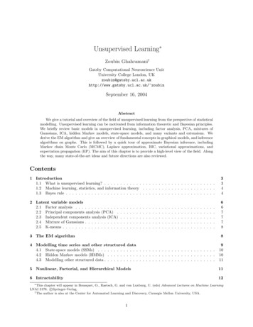
Locality Sensitive Hashing In ‘conventional’ hashing, similarities between datapointsare not conserved. LSH is a way to produces hashes that can be comparedwith a similarity function. The hash function is a projection matrix defining a randomhyperplane. If the projected datapoint v falls on one side ofthe hyperplane, its hash h( v ) 1, otherwise h( v ) 1.27
Locality Sensitive HashingImage from VanDurme & Lall (2010): http://www.cs.jhu.edu/ vandurme/papers/VanDurmeLallACL10-slides.pdf28
Locality Sensitive HashingImage from VanDurme & Lall (2010): http://www.cs.jhu.edu/ vandurme/papers/VanDurmeLallACL10-slides.pdf(The Hamming distance between two strings of equal length is the number of positions at whichthe symbols differ across strings.)29
Doing LSH over a semantic space The hash value of an input point in LSH is made of all the projections onall chosen hyperplanes:Mp n Rn k Sp k Say we have k 10 hyperplanes h1 .h10 (the columns of matrix R) and we are projecting the vector dog with dimensionality n 300 on thosehyperplanes: dimension 1 of the new vector is the dot product of dog andPh1 :dogi h1i dimension 2 of the new vector is the dot product of dog andPh2 :dogi h2i . We end up with a ten-dimensional vector which is the hash of dog.30
Interpretation of the LSH hash Each hyperplane is a discriminatory feature cutting throughthe data. Each point in space is expressed as a function of thosehyperplanes. We can think of them as new ‘dimensions’ relevant toexplaining the structure of the data. Random indexing is ‘random’ because the matrix Rn k isobtained by sampling vectors (hyperplanes) from aGaussian distribution, in a way that each one is orthogonalto the others.31
Random Indexing: incremental LSH A random indexing space can be simply and incrementallyproduced through a two-step process:1. Map each context item c in the text to a random projectionvector (to get R).2. Initialise each target item t as a null vector. Whenever weencounter c in the vicinity of t we update t t c . The method is extremely efficient, potentially has lowdimensionality (we can choose the dimension of theprojection vectors), and is fully incremental.32
Relating vector addition to random projection We said that LSH used a random projection matrix so thatMp n Rn k Sp k Here’s a toy example.t1t2c1 21rc2 3 0 c1 1 c20!30 So we have two random vectors (0) and (1) corresponding to contexts c1 and c2 . We got 3 by computing 2 0 3 1 This is equivalent to computing (0 0) (1 1 1) So we added the random vectors corresponding to each context for eachtime it occurred with the target. That’s incremental random indexing.33
Is RI human-like? Not without adding PPMI weighting at the end of the RIprocess. (This kills incrementality.)QasemiZadeh et al (2017)34
Clustering35
Clustering algorithms A clustering algorithmpartitions some objectsinto groups namedclusters. Objects that are similaraccording to a certain setof features should be in thesame cluster.From alysis-in-r-practical-guide/36
Why clustering Example:1 we are translating from French to English, andwe know from some training data that: Dimanche on Sunday ; Mercredi on Wednesday ; What might be the correct preposition to translate Vendrediinto the English Friday ? (Given that we haven’t seen itin the training data.) We can assume that the days of the week form a semanticcluster, which behave in the same way syntactically. Here,clustering helps us generalise.1Example from Manning & Schütze, Foundations of statistical language processing.37
Flat vs hierarchical clusteringFlat clusteringHierarchical clusteringFrom nalysis-in-r-practical-guide/38
Soft vs hard clustering In hard clustering, each object is assigned to only onecluster. In soft clustering, assignment can be to multiple clusters,or be probabilistic. In a probabilistic setup, each object has a probabilitydistribution over clusters. P(ck xi ) is the probability thatobject xi belongs to cluster ck . In a vector space, the degree of membership of an objectxi to each cluster can be defined by the similarity of xi tosome representative point in the cluster.39
Centroids and medoids The centroid or center of gravity of a cluster c is theaverage of its N members:µk 1 XxN x ck The medoid of a cluster c is a prototypical member of thatcluster (its average distance to all other objects in c isminimal):xmedoid argminy {x1 ,x2 ,··· ,xn }nXd(y , xi )i 140
Hierarchical clustering: bottom-up Bottom-up agglomerative clustering is a form ofhierarchical clustering. Let’s have n datapoints x1 .xn . The algorithm functions asfollows: Start with one cluster per datapoint: ci : {xi }. Determine which two clusters are the most similar, andmerge them. Repeat until we are left with only one cluster C {x1 .xn }.41
Hierarchical clustering: bottom-upNB: The order in which clusters are merged depends on the similarity distributionamongst datapoints.42
Hierarchical clustering: top-down Top-down divisive clustering is the pendent ofagglomerative clustering. Let’s have n datapoints again: x1 .xn . The algorithm relieson a coherence and a split function: Start with a single cluster C {x1 .xn } Determine the least coherent cluster and split it into twonew clusters. Repeat until we have one cluster per datapoint: ci : {xi }.43
Coherence Coherence is a measure of the pairwise similarity of a setof objects. A typical coherence function:Coh(x1.n ) mean{Sim(xi , xj ), ij 1.n, i j} E.g. coherence may be used to calculate the consistencyof topics in topic modelling.44
Split We need a heuristic to split a cluster into two new clusters. Take the point with the maximum distance to all otherpoints in the cluster cn and make it a new cluster cn 1 . Move all points in cn which are more similar to cn 1 .45
Similarity functions for clustering Single link: similarity of two most similar objects acrossclusters. Complete link: similarity of two least similar objectsacross clusters. Group-average: average similarity between objects.(Here, the average is over all pairs, within and acrossclusters.)46
Effect of similarity functionClustering with single linkGraph taken from Manning, Raghavan & ctures/lecture12-clustering.pdf47
Effect of similarity functionClustering with complete linkGraph taken from Manning, Raghavan & ctures/lecture12-clustering.pdf48
K-means clustering K-means is the main flat clustering algorithm. Goal in K-means: minimise the residual sum of squares(RSS) of objects to their cluster centroids:XRSSk x µk 2x ck The intuition behind using RSS is that good clusters shouldhave a) small intra-cluster distances; b) large inter-clusterdistances.49
K-means algorithmSource: https://en.wikipedia.org/wiki/K-means clustering50
Convergence Convergence happens when the RSS will not decreaseanymore. It can be shown that K-means will converge to a localminimum, but not necessarily a global minimum. Results will vary depending on seed selection.51
Initialisation Various heuristics to ensure good clustering: exclude outliers from seed sets; try multiple intialisations and retain the one with lowestRSS; obtain seeds from another method (e.g. first do hierarchicalclustering).52
Number of clusters The number of clusters K is predefined. The ideal K will minimise variance within each cluster aswell as minimise the number of clusters. There are various approaches to finding K . Examples thatuse techniques we have already learnt: cross-validation; PCA.53
Number of clusters Cross-validation: split the data into random folds andcluster with some k on one fold. Repeat on the other folds.If points consistently get assigned to the same clusters (ifmembership is roughly the same across folds) then k isprobably right. PCA: there is no systematic relation between principalcomponents and clusters, but heuristically checking howmany components account for most of the data’s variancecan give a fair idea of the ideal cluster number.54
Evaluation of clustering Given a clustering task, we want to know whether thealgorithm performs well on that task. E.g. clustering concepts in a distributional space: cat andgiraffe under ANIMAL, car and motorcycle under VEHICLE(Almuhareb 2006) Evaluation in terms of ‘purity’: if all the concepts in oneautomatically-produced cluster are from the samecategory, purity is 100%.55
Purity measure Given a cluster k and a number of classes i, purity isdefined asP(Ck ) 1maxi (nki )nk Example: given the cluster C1 {A A A T A A A T T A}:1max(7, 3) 0.710 NB: here, the annotated data is only used for evaluation,not for training!! (Compare with k-NN algorithm.)P(C1 ) 56
Clustering in real life57
fundamental to NLP: dimensionality reduction (e.g. PCA, using SVD or any other technique); clustering; some neural network architectures. 2. Dimensionality reduction 3. Dimensionality reduction Dimensionality reduction refers to a set of techniques used to reduce the number of variables in a model. For instance, we have seen that a count-based .