Transcription
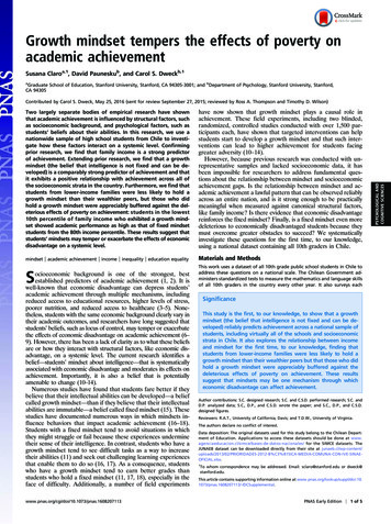
Image to LatexGuillaume GenthialStanford UniversityICMERomain SauvestreStanford d.eduAbstractaccuracy to understand hand written text and render itfrom images. Hence, the next step towards renderinghand-written mathematical notes into a LATEX documentis to teach computers to reconstruct the LATEX code thatgenerates a given formula. This task differ from standardOptical Character Recognition (OCR) techniques by thecomplexity of the underlying syntax and is closer toimage captioning than standard OCR. To this purpose, wecan leverage image captioning techniques to address thistask. Our system would take as input a formula (the image) and would generate a list of LATEX tokens (the caption).Converting images of mathematical formulas to LATEXcode is a problem that combines challenges both from computer vision and natural language processing, close to therecent breakthroughs in image captioning. Such a systemwould be very useful for people using LATEX in their everyday life such as students or researchers. We addressed thistask with a dual setting encoder-decoder, combined with anattention mechanism. This model is trained on a 100, 000LATEX formulas scraped from ArXiv. We evaluate our modelagainst several metrics, both at the code level (perplexity,exact match, BLEU score .) and at the image level (Levenshtein distance, exact match) by compiling the predictedcode to generate new formulas and comparing them to theground truth. We achieve very good performance with aBLEU score of 78% and an image edit-distance of 62%.Image captioning is a surging field of deep learning thathas gotten more and more attention in the past few years,being at the crossroads between computer vision and NLP.This is one of the main attempts to combine these two fieldsof machine learning, to achieve more general artificial intelligence with machines being able to both see and speakat the same time. The current state of the art in imagecaptioning has a similar approach as sequence to sequencemodels described by [Sutskever et al., 2014]: first we encode the input image in a fixed size vector and then decode this vector by generating tokens from the caption oneafter the other. Adding an attention mechanism was alsoproved to greatly enhance the performance of these models[Luong et al., 2015] (cf Figure 1).1. IntroductionRecently, 20,000 handwritten notes of AlexanderGrothendiek, one of the greatest mathematician of the 20thcentury, were scanned and released by the University ofMontpellier, making it available to every researcher inthe world as it is believed it could advance research inmany fields of mathematics. However, reading these notesis not only a challenge due to their very high theoreticalcomplexity, but also because they are not written in a properformat. We can imagine that they would get more attentionand research interest if they were nicely computerized ina clean LATEX document, which would incentivize moreresearchers to peak into the work of one of the greatestgeniuses of the past century. However, it would takeyears for a human to type all these notes on LATEX, themost challenging part being to understand and type all themathematical equations.Figure 1. Generating[Deng et al., 2016]LATEXfromimages,figurefromLittle attention has been given to its applicationto reconstructing LATEX code from mathematical formulas. OpenAi listed this problem in their blog asa request for research ( https://openai.com/Recent breakthroughs in computer vision and NaturalLanguage Processing (NLP) could address this challenge.Computers are already able to achieve almost perfect1
requests-for-research/#im2latex)andearlier last year, a team from Harvard University[Deng et al., 2016] proposed an attention-based modelto address this issue. Note that due to the fact that differentformulas can produce similar or same images add a complexity to the task, compared to standard image captioning.It also raises issues about the evaluation of such models.In this project, we combine the approach of[Deng et al., 2016] and the image captioning systemof [Xu et al., 2015] and build on their models to improvethe results. Our main contributions are:Combining sequence-to-sequence with Image Captioning techniques, [Xu et al., 2015] encode the image in a fixedsize vector with a CNN, and then decoding the vector stepby step, generating at each step a new word of the captionand feeding it as an input to the next step. In their work, theyalso added an attention mechanism, enabling the decoder ateach time step to look and attend at the encoded image, andcompute a representation of this image with respect to thecurrent state of the decoder (Figure 2). a fully end-to-end LATEX rendering system that couldalso be applied to image captioning, and more globallyto any image-to-text problem. a comparison between different encoders and decodersas well as an analysis of the performance of an imagecaptioning model on this particular problem.2. Related WorkFigure 2. Attention based model for image captioning, figure from[Xu et al., 2015]In the past few years, lots of breakthroughs havetaken place in Computer Vision, originated by the performance of [Lecun et al., 1998]’s system to recognizedigits. Optical Character Recognition has since gainedinterest, with highly-accurate systems like the one of[Ciresan et al., 2010]. On the task of recognizing mathematical expressions that introduces new challenges of grammar understanding, some attempts have managed to buildsystems by exploiting character segmentation and grammar reconstruction, like [Miller and Viola, 1998], or othersyntactic-based approaches like [Chan and Yeung, 2000]and [Belaid and Haton, 1984].Techniques combining neural network and standard NLP approaches likeConditional Random Field have also proven to bevery effective to recognize words in images like in[Jaderberg et al., 2014], or using convolutional neural networks like in [Wang et al., 2012].In Natural Language Processing, sequence-tosequence models based on recurrent neural networkshave forged ahead in the race to machine translation[Sutskever et al., 2014], improving by a lot the quality oftranslation from one language to another. The introductionof attention by [Bahdanau et al., 2014] [Luong et al., 2015]eventually established a new standard in Machine Translation systems, allowing impressive performance likezero-shot translation like in [Johnson et al., 2016].Advances have also been made in Image Captioning,using recurrent neural network for the most part, like in[Karpathy et al., 2015]. [Karpathy and Li, 2014] proposedto learn a joint embedding space for ranking and generationwhose model learns to score sentence and image similarityas a function of R-CNN object detections with outputs of abidirectional RNN.Recent work from [Deng et al., 2016] took this sameapproach and successfully applied it to the generation ofLATEXcode from images of formulas. They used the samemechanism of soft attention as in [Luong et al., 2015], andwere able to achieve as much as 77% of exact match scoreon the test dataset.3. ModelThe architecture of our model is an adaptation Show, Attend and Tell [Xu et al., 2015] for LATEX code generationthat we combine with some details of [Deng et al., 2016]work.3.1. Encoder-DecoderThe main building block of our model is based on theencoder-decoder framework.Encoder First, we encode the images with a convolutionneural network that consists of 6 convolution layers withfilters of size 3x3, stride of 1 and padding of 1. After theconvolution layers we also add max pooling layers. Therole of these max-pooling is to extract structure from thecharacters. See details of the architecture of the network onFigure 3.This CNN encodes the original image of size H x W intoa feature map of size H’ x W’ x C where C is the numberof filters of the last convolution layer. The encoder definesone vector vi RC for each of the H’ x W’ regions. Intu2
itively, each vi captures the information from one region ofthe image.ct Att(ht , V )ot tanh(W c [ht , ct ])p(yt 1 y1 , ., yt , ) sof tmax(W out ot )where E is an embedding matrix, and W are matrices.Note that here ct stands for the attention vector (or context vector, see Section 3.2), and not the cell state of theLSTM (the cell state is not represented in these equationsbut is inherent to the LSTM cell). V is the encoded image.We use two special tokens START and END. Once ourdecoder predicts the END token, we stop generating newtokens. The START token is used to initialize the decoder. Instead of initializing hidden vectors to zeros like in[Deng et al., 2016], we combine with the more expressiveinitialization from [Xu et al., 2015] and each hidden state isinitialized with the following rule h0 tanh Wh · 1H 0 xW 00HXxW 0 v i bh i 1where we learn an independent matrix Wh and bias bhfor each of the hidden states (including the memory of theLSTM and the output vector ot ).Figure 3. Convolutional Encoder3.2. Attention mechanismTo enhance the performance of the decoder, we add asoft attention mechanism as it was proved to help convergence in the case of image captioning [Xu et al., 2015].Hence, at each time step of the decoding process, our RNNattends to the feature map V and compute a weighted average of these vectors. We used the following attention mechanism from Mannings et. al [Luong et al., 2015]:Decoder Once we have a feature map of size H’ x W’ xC, (in other words H’ x W’ vectors vi RC ) we can decode this representation of the image to produce the LATEXtokens with a recurrent neural network. For this task,LSTMs ([Hochreiter and Schmidhuber, 1997]) have shownto be very efficient to capture long term dependencies andfacilitate the back-propagation of gradients.Formally, our decoder takes as input a hidden vectorht 1 (the hidden state of the LSTM, that include both thehidden state and the memory) and takes as input the previous token yt 1 . At each time step, the decoder computesan attention vector (see Section 3.2) ct that depends on theimage and the next hidden vector.It then produces a distribution over the next token with arecursive formulaeti β T tanh(Wh ht 1 W vi )αt sof tmax(et )tc 0HX W 0αit vii 13.3. Beam searchAt each time step, the LSTM produces a vector yt ofdimension V that is the size of the vocabulary and that represents the distribution probability over the vocabulary forthe next word. From the vector yt we need to decide whichtoken to output and feed as input to the next step. We triedtwo different approaches to solve this problem:p(yt ) f (yt 1 , ht 1 , ct )More specifically, we also compute another outputstate ot used to compute the distribution probabilityover the vocabulary. This implementation is similar to[Deng et al., 2016] and differs from [Xu et al., 2015]. Thedetails of the recurrent step are as follows Greedy approach: the simplest approach is to simplyoutput the token that has the highest probability at eachtime step. We refer to this approach as being greedyht LST M (ht 1 , [Eyt 1 , ot 1 ])3
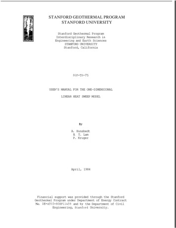
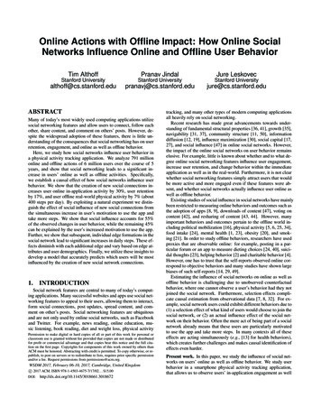
because it can be suboptimal. For instance when looking for an optimal path in a graph to maximize the rewards on the edges of the graphs, the greedy approachis to take at each node the edge with he highest reward.However this technique can be suboptimal and lead toa lower reward at the end. Beam search: to try to bridge the gap that can existbetween the greedy solution and the optimal solution,we implemented a beam search method to find the optimal output sentence. Now, at each time step we keepin memory the B hypotheses (sequence of tokens) withthe highest probability, B being the beam size (e.g. B 5). At each time step we input the B tokens to thedecoder, compute B vector yt and then update the listof tokens that we keep while keeping track of the ”parents” of the B tokens with the highest probability overthe B vectors yt . What we want to maximize over thetime steps of decoding is the product of probabilitiesof each token in a sentence given its parent. Hence, wecan reconstruct the optimal sentence at the end of thedecoding process and output our ”optimal” sentence.Note that B 1 is equivalent to the greedy approach.This method would be more robust to an mispredictedlabel at some time step.Figure 4. Formula LengthWe train our network to maximize the probability of thereference formula.4.2. Preprocessing stepsFirst we need to preprocess the images and formulas before we can input them to our model: Images: Each image is rendered using pdflatexand the magick tools.We use parameters-density 200 and downsample images by a factor2. On top of this, we use a greyscale representation.This way, the input to our network are low resolutionimages with just enough information to recognize thecharacters (readable by a human eye, but barely). Thetypical size is 200 x 160 pixels. We transfer the data onGPU using uint8 to save on the CUDA Memcpy. Tomake the training go faster, we form buckets of imagesof the same shape (x2 speedup).4. Dataset and Training4.1. Dataset and ImplementationOur main dataset is the prebuilt dataset from[Deng et al., 2016], im2latex-100k, that includes a total of 100k formulas and images splitted into train( 84k), validation ( 9k) and test ( 10k) sets. Formulas were parsed from LATEX articles on arXiv (https://zenodo.org/record/56198#.WP1ksdI182x).We note that this problem is particularly difficult as roughlyhalf of the formulas contain more than 50 tokens! (SeeFigure 4). In the seq-to-seq setting, as the generated tokensdepends on the beginning of the sentence and the previoustokens, this is a particular challenge!We decided to limit the scope of this project to PDF images and not to treat the case of hand-written formulas. Anextension of this work could be to run the same model usingthe CROHME dataset (not a typo!) that consists of 10,000handwritten mathematical expressions and their LATEXcode.We implemented our models using Tensorflow andrun our experiment on a Tesla K80. We release the code forour own attention wrapper and Beam Search, as these functionalities are to be part of the next release version (and notyet implemented). 1 We use 15 epochs for a training timeon the whole dataset of 12 hours. Our code is roughly twiceas fast as the lua implementation of [Deng et al., 2016]. Formulas: We tokenize the formulas as it as beenobserved that token-based methods are more efficientthan character-based. We use the preprocessing scriptsof [Deng et al., 2016] that uses Katex, a LATEX parserwritten in javascript. Once the formulas are tokenized,we form our vocabulary of size 509 to which weadd the special tokens ”PAD”, ”START”, ”END”, and”UNK” that represent the padding tokens, the start/endof sentence token and the unknown token respectively.We then pad the formulas with the ” PAD” token tomake sure that they all have the same length (maximum length of 150) when we input them to our recurrent neural network. We build on [Deng et al., 2016]findings and use normalized LATEX when possible.(This forces the use of conventions like x {i} insteadof x i.)4.3. Parameters and Optimization1 Thecode is available here https://github.com/guillaumegenthial/image2latexWe used the following hyper-parameters for our model4
Text-based First, we relied on widely used metrics inNatural Language Processing such as exact match, perplexity and BLEU score ([Papineni et al., 2002]). The exactmatch quantity between a predicted formula and groundtruth formula is one if the tokens of both formulas are exactly the same (same order, same number and same nature).The perplexity of a language tries to capture how confident(or confused) the model is at predicting one token. The perplexity of a language model is defined as1perplexity e NFigure 5. Learning rate schedule with warm-up - log scalePNi 1log(xi )where N is the total number of tokens to predict in the wholedataset, and xi is the predicted probability of the true tokeni. For instance, when the model is completely random, theperplexity will be the number of words in the vocabulary V,meaning that for every word to predict, the model hesitatesbetween V words. Conversely, a very good model shouldachieve a perplexity close to 1 meaning that the model isvery confident in predicting the true word. We also used theBLEU score that captures the overlap of n-grams, as it hasbeen shown to be the most correlated with human judgmentand it is thus a standard metric in translation (1 is perfect).Finally, we can also compute the edit distance on the text(Levenshtein distance), between the predicted formula andthe ground truth. This distance between two strings tellsus how many characters we should add/remove/change inone string to obtain the other one. We report the edit distance which is the percentage of the reconstructed text thatmatches the original. Thus, a perfect match has an edit distance of 1.Image-based LSTM dim: 512 Embeddings: 80 Batch-size: 20 (limited by the GPU memory) Max length: we use a default max of 150 tokens unless specified otherwise. Learning-rate: training attention based seq-toseq models has been shown to be hard to train.We obtained good results with Adam optimizer([Kingma and Ba, 2014]). As some runs were unableto learn, we used the warm-up strategy as mentionedby [Goyal et al., 2017]. Due to high variance and highgradients at the beginning of the training, we use asmall warm-up learning rate of 1e-4 for the two firstepochs. Then, we use a constant learning rate of 1e-3until the 10-th epoch where we start to decay exponentially until 1e-5 at the end of the 15-th epoch. Thisstrategy highly improved both the quality of our resultsand the speed of training compared to a constant or exponentially decaying schedule. See Figure 5. Beam size: 5 yielded good performance. Weights initialization: we use orthogonal initialization for embeddings and recurrent matrices, other wisewe use the default Xavier initialization. Orthogonalmatrices helped stabilize the training.4.4. EvaluationTo evaluate the performance of the model, we must firstunderstand that LATEX is not a normalized language: different codes can still generate the same formula when compiled. For instance, the brackets are not always mandatoryand ”xˆ2” or ”xˆ{2}” will still produce the same formulason a PDF. We study two types of metrics to evaluate ourmodel: one based on how well we reproduce the LATEX code,one based on how well the reconstructed image is close tothe original.Figure 6. Edit distance on imagesHowever, all these evaluation metrics do not take intoaccount the problem of non normalization of LATEX, and we5
DecodingGreedyBeam search (prediction)Beam search (best proposal)[Deng et al., 2016] CNNEncEM Img0.220.320.350.53BLEU0.760.780.780.75Edit text0.760.760.76NREdit Image0.350.620.620.61Table 1. Comparison of beam search with greedy decoder and the equivalent model from [Deng et al., 2016] (CNNEnc). We obtain similarperformance on most of the metrics, except for the Exact Match where CNNEnc obtains a much higher score.might underestimate our model if we only rely on these metrics. This is why we also implemented an evaluation metricon the images generated from the predicted formulas, calledthe edit distance for images (or Levenshtein distance for images). Figure 6 depicts the method we apply to computethis distance over images. First we split the image in several columns and we encode each column with an integer.Slicing the images makes sense at the expression level anddoes not dilute distance like a pixel-wise distance would.From the Levenhstein distance between the columns of thereference and the predictions, we can compute a percentageof columns that are the same. We report his edit distance.1 means that we have an exact match.Figure 7. Distribution of Edit distancesdistribution on Figure 8. As expected, the first hypothesis isalmost always the best one, but if a user were proposed thefew proposals, we could gain some performance.5. ExperimentsGeneral [Deng et al., 2016] use a more complex architecture for the encoder with an recurrent additional layer to extract temporal dependencies in the image. We first comparethe performance of their equivalent model (simple CNN encoder) with ours on the full dataset (all formula lengths).We obtain similar results except for the exact match distance. It may be due to the fact that we have a hard thresholdof zero-difference between 2 images to count it as an exactmatch, but [Deng et al., 2016] may use a softer thresholdthat would explain the discrepency in the results.Otherwise, we notice that beam search is slightly moreefficient than greedy decoding in term of Exact Matches(0.35 instead of 0.32). Due to the clever initialization ofthe hidden states our model is able to slightly outperformthe CNNEnc of [Deng et al., 2016]. It is important to notethat their model contains more parameters than ours (theyadd unspecified parameters in the convolutions). Thus ourmodel is both lighter, faster and equivalently efficient.Interestingly, Figure 7 shows that while there is a continuous distribution of the formulas (Text) edit distance, mostof the formulas are perfectly rendered. This suggests thatchanges in LATEX do not necessarily induces big changes inthe rendered formula, as expected. We also see that ourmodel does a pretty good job at rendering images! Figure 5presents some examples of mistakes.We also point out the usefulness of the beam-search thatproduces multiple proposals. If we have a look at whichof the proposal matches the best the reference, we find theFigure 8. Distribution of Edit distancesDropout We tried to add dropout to our model to avoidover-fitting but as we can see in the table below the bestperforming model is still the one with no dropout. However,these results are subject to caution as we evaluated it onlyon the half of the dataset. We applied the dropout like in[Xu et al., 2015].6
Dropout00.20.5EM0.210.20.16BLEU0.800.780.75Edit text0.830.820.80Edit Image0.740.660.63Table 2. Comparison of models with different dropouts on a subsetof the dataset - formulas with less than 50 tokens - 36k examplesEmbeddings Our model initializes the embeddings of thetoken randomly. We tried to train embeddings in an unsupervised manner using CBOW ([Mikolov et al., 2013]).However, we would need a lot more data to build interestingrepresentation, that could constitute itself a paper but morefocused on the NLP side. We didn’t notice any improvement in performance.Encoders As [Deng et al., 2016] noticed some improvement using a bi-LSTM encoder on top of the CNNEnc, wetried to add more parameters and remove the destructivemax-pool layers from the network. Following the intuitionof the recent paper [Gehring et al., 2017], we replace thesemax-pool by an additional convolutional layer with a biggerfilter and an equivalent stride (thus the output of the encoderhas the same shape as our previous encoding). The architecture of this network is represented on Figure 9.We also evaluated the impact of adding residual connections between the convolutional layers (see our code formore 0.31BLEU0.800.780.84Edit text0.830.81–Figure 9. Variation of the EncoderEdit Image0.740.66–Figure 10. Performance of our model as a function of the formulalengthTable 3. Comparison of models with different encoders on the formulas with less than 50 tokens. Our variation seems to achievemuch higher results (some metrics are still missing). ResidualConnection do not seem to help, on the contrary[Gehring et al., 2017]) and our own experiments suggestthat it might be a computational waste (bi-LSTM are notas parallelizable as CNN). Future work could even incorporate a CNN-based decoder like in [Gehring et al., 2017],with the advantage of being much faster at training time.Influence of Formula Length As expected, the longerour sentences, the lower the performance. See 10. In longsentence, the model is more prone to attention errors butalso is sensible to errors while decoding.References[Bahdanau et al., 2014] Bahdanau, D., Cho, K., and Bengio, Y.(2014). Neural machine translation by jointly learning to alignand translate. CoRR, abs/1409.0473.6. Conclusion[Belaid and Haton, 1984] Belaid, A. and Haton, J.-P. (1984).A syntactic approach for handwritten mathematical formularecognition. IEEE Trans. Pattern Anal. Mach. Intell., 6(1):105–111.This paper presents an efficient implementation of acaption-generation system applied to LATEX generation fromraw images. We obtain good performance, similar to[Deng et al., 2016]. As outlined in the experiments, theencoder might be improved. If [Deng et al., 2016] obtaingood results with a bi-LSTM, more recent papers (like[Chan and Yeung, 2000] Chan, K.-F. and Yeung, D.-Y. (2000).Mathematical expression recognition: a survey. InternationalJournal on Document Analysis and Recognition, 3(1):3–15.7
TruthPredictionBestTable 4. Examples of mistakes. We render the predicted formula to compare with the original image using pdflatex - The entry bestshows the best hypothesis among the beam search proposal if different from the first proposal. Among these examples, we notice that someof the mistakes are minor mistakes and that it can happen that the best proposal from the beam search is not the first one.[Ciresan et al., 2010] Ciresan, D. C., Meier, U., Gambardella,L. M., and Schmidhuber, J. (2010). Deep big simple neural netsexcel on handwritten digit recognition. CoRR, abs/1003.0358.[Mikolov et al., 2013] Mikolov, T., Chen, K., Corrado, G., andDean, J. (2013). Efficient estimation of word representations invector space. CoRR, abs/1301.3781.[Deng et al., 2016] Deng, Y., Kanervisto, A., and Rush, A. M.(2016). What you get is what you see: A visual markup decompiler. CoRR, abs/1609.04938.[Miller and Viola, 1998] Miller, E. G. and Viola, P. A. (1998).Ambiguity and constraint in mathematical expression recognition. In Proceedings of the Fifteenth National Conference onArtificial Intelligence and Tenth Innovative Applications of Artificial Intelligence Conference, AAAI 98, IAAI 98, July 26-30,1998, Madison, Wisconsin, USA., pages 784–791.[Gehring et al., 2017] Gehring, J., Auli, M., Grangier, D., Yarats,D., and Dauphin, Y. N. (2017). Convolutional sequence to sequence learning. CoRR, abs/1705.03122.[Papineni et al., 2002] Papineni, K., Roukos, S., Ward, T., andZhu, W.-J. (2002). Bleu: A method for automatic evaluation ofmachine translation. In Proceedings of the 40th Annual Meeting on Association for Computational Linguistics, ACL ’02,pages 311–318, Stroudsburg, PA, USA. Association for Computational Linguistics.[Goyal et al., 2017] Goyal, P., Dollár, P., Girshick, R., Noordhuis,P., Wesolowski, L., Kyrola, A., Tulloch, A., Jia, Y., and He, K.(2017). Accurate, Large Minibatch SGD: Training ImageNetin 1 Hour. ArXiv e-prints.[He et al., 2015] He, K., Zhang, X., Ren, S., and Sun, J. (2015).Deep residual learning for image recognition. CVPR.[Sutskever et al., 2014] Sutskever, I., Vinyals, O., and Le, Q. V.(2014). Sequence to sequence learning with neural networks.NIPS.[Hochreiter and Schmidhuber, 1997] Hochreiter, S. and Schmidhuber, J. (1997). Long short-term memory. Neural Comput.,9(8):1735–1780.[Jaderberg et al., 2014] Jaderberg, M., Simonyan, K., Vedaldi, A.,and Zisserman, A. (2014). Deep structured output learning forunconstrained text recognition. CoRR, abs/1412.5903.[Wang et al., 2012] Wang, T., Wu, D. J., Coates, A., and Ng, A. Y.(2012). End-to-end text recognition with convolutional neuralnetworks. In Proceedings of the 21st International Conferenceon Pattern Recognition (ICPR2012), pages 3304–3308.[Johnson et al., 2016] Johnson, M., Schuster, M., Le, Q. V.,Krikun, M., Wu, Y., Chen, Z., Thorat, N., Viégas, F. B., Wattenberg, M., Corrado, G., Hughes, M., and Dean, J. (2016).Google’s multilingual neural machine translation system: Enabling zero-shot translation. CoRR, abs/1611.04558.[Xu et al., 2015] Xu, K., Ba, J., Kiros, R., Cho, K., Courville,A. C., Salakhutdinov, R., Zemel, R. S., and Bengio, Y. (2015).Show, attend and tell: Neural image caption generation withvisual attention. CoRR, abs/1502.03044.[Karpathy et al., 2015] Karpathy, A., Johnson, J., and Li, F.(2015). Visualizing and understanding recurrent networks.CoRR, abs/1506.02078.[Karpathy and Li, 2014] Karpathy, A. and Li, F. (2014). Deepvisual-semantic alignments for generating image descriptions.CoRR, abs/1412.2306.[Kingma and Ba, 2014] Kingma, D. P. and Ba, J. (2014). Adam:A method for stochastic optimization. CoRR, abs/1412.6980.[Lecun et al., 1998] Lecun, Y., Bottou, L., Bengio, Y., andHaffner, P. (1998). Gradient-based learning applied to document recognition. In Proceedings of the IEEE, pages 2278–2324.[Luong et al., 2015] Luong, M.-T., Pham, H., and Manning, C. D.(2015). Effective approaches to attention-based neural machinetranslation. EMNLP.8
a clean LATEX document, which would incentivize more researchers to peak into the work of one of the greatest geniuses of the past century. However, it would take years for a human to type all these notes on LATEX, the most challenging part being to understand and type all the mathematical equations. Recent breakthroughs in computer vision and .