Transcription
Document de Recherche du Laboratoire d’Économie d’OrléansWorking Paper Series, Economic Research Department of the University of Orléans (LEO), FranceDR LEO 2018-03The (low) fiscal multiplierwhen debt is denominated inforeign currencyMarie-Pierre HORYGrégory LEVIEUGEDaria ONORIMise en ligne / Online : 04/11/2019Remplace une version précédente du même numéro / Replaces a previous version of the same DR LEO numberCette version remplace celle du / This replaces the previous version dated : 18/12/2018Titre précédent / A previous version was titled : "Foreign currency denominated debtand the fiscal multiplier ”Laboratoire d’Économie d’OrléansCollegium DEGRue de Blois - BP 2673945067 Orléans Cedex 2Tél. : (33) (0)2 38 41 70 37e-mail : leo@univ-orleans.frwww.leo-univ-orleans.fr/
The (low) fiscal multiplier when debt is denominated inforeign currencyMarie-Pierre Hory†Grégory Levieuge‡Daria Onori§November 2019AbstractThis paper aims to explain why fiscal multipliers are generally low, even close tozero, in emerging economies (EMEs). Our explanation jointly relies on the behaviorof the exchange rate following a fiscal shock and on the proportion of external debtdenominated in foreign currency, which is usually important in EMEs. According tothe recent literature, the real exchange rate can depreciate following an increase inpublic spending. If this is the case, the debt burden denominated in foreign currencyincreases, and the domestic firms’ balance sheets deteriorate, raising their external finance premium and further crowding out private investment. Finally, this phenomenonmay offset the initial crowding-in impact of the public spending shock. We demonstratethat such an explanation is theoretically valid: the higher the share of external debtdenominated in foreign currency is, the lower the fiscal multiplier.JEL Classification: E62; F34; F41Keywords: Fiscal multiplier; DSGE; Currency mismatch; Financial frictions; EmergingcountriesThe views expressed in the article are those of the authors and do not necessarily reflect those of theBanque de France.†ISC Paris and Univ.Orléans, CNRS, LEO, FRE 2014, F-45067, France.E-mail address:mphory@iscparis.com.‡Corresponding author. Banque de France, DGEI-DEMFI-RECFIN (041-1391); 31, rue Croix des PetitsChamps, 75049 Paris Cedex 01 France, and Univ. Orléans, CNRS, LEO, FRE 2014, F-45067, France. E-mailaddress: gregory.levieuge@banque-france.fr.§Univ. Orléans, CNRS, LEO, FRE 2014, F-45067, France. E-mail address: daria.onori@univ-orleans.fr.
1IntroductionThe global economy has entered a synchronized slowdown, concerning most of the countries in the world. In this context, many economists in line with the International MonetaryFunds consider that it is time for countries with fiscal space to deploy “fiscal firepower” toboost demand and growth potential. Given their low level of public debt1 , emerging countriesin particular may rely on fiscal stimulus. However, empirical evidence suggests that fiscalmultipliers are significantly smaller in emerging market economies (EMEs), where they areusually found to be close to zero, compared to advanced countries (AEs).2In this paper, we provide an explanation for the difference between fiscal multipliers inEMEs and AEs, which is based on the currency denomination of external debt. As shown inFigure 1, the share of foreign currency denominated external debt in EMEs is approximatelythree times higher than that in AEs.3 Combined with the reaction of the exchange rate following a public spending stimulus, this large difference may be a source of diverging multipliereffects. Indeed, contrary to the textbook Mundell-Fleming-Dornbush model, several recentpapers show that the domestic currency depreciates following a domestic increase in publicspending (Betts and Devereux, 2000; Kollmann, 2010; Corsetti et al., 2012a; Bouakez andEyquem, 2015). Thus, because of adverse balance sheet effects due to a currency mismatch,the depreciation of the domestic currency may eventually be contractionary (Céspedes et al.,2004).4 This phenomenon may offset the initial crowding-in impact of the public spendingshock.Generally, the literature shows that fiscal multipliers are larger when public debt is low(Cimadomo et al., 2010; Ilzetzki et al., 2013; Nickel and Tudyka, 2014), under fixed exchangerate regimes (Born et al., 2013; Corsetti et al., 2012a), during business cycle downturns(Gechert and Rannenberg, 2018) and when interest rates are relatively low.5 The level ofdevelopment is also considered a determinant per se, albeit without explaining why fiscalmultipliers are so small in EMEs. Actually, none of the aforementioned determinants canexplain the fiscal multiplier differential. For example, emerging countries often experimentwith lower public debt-to-GDP ratios than AEs, which should lead to larger multiplier effects.1Considering a panel of 41 countries from Europe and Central Asia between 2000 and 2013, the averagedebt-to-GDP ratio is 54% for high income countries, compared to 34% for middle income countries (source:Historical Public Debt Database, International Monetary Fund).2See, for example, Ilzetzki et al. (2013); Hory (2016); Chian Koh (2017).3Source: World Bank, Quarterly external debt statistics. Due to a lack of financial accounts data in manyEMEs, analyses of currency mismatches are scarce. For recent assessments of risks related to cross-borderlending, see Chui et al. (2014), Catão and Milesi-Ferretti (2014) and Chow (2015).4This is a reason why many central banks are reluctant to allow their currencies to devalue in responseto external shocks. See, for instance, Hausmann et al. (2001) and Calvo and Reinhart (2002).5See, for instance, Woodford (2011); Christiano et al. (2011); Nakamura and Steinsson (2014); Giambattista and Pennings (2017). See Bilbiie et al. (2019) for an opposite view.1
Figure 1: Share of foreign currency denominated external debtCertainly, the low fiscal efficiency in EMEs may be due to some particularities such as aless-flexible supply side and inefficient management of public spending. However, we demonstrate that our complementary - while not not necessarily exclusive - explanation based onboth the behavior of the exchange rate following a fiscal shock and on the foreign currency denomination of private debt is theoretically valid in a two-country dynamic stochastic generalequilibrium (DSGE) model with incomplete and imperfect international financial markets,sticky prices, external indebtedness and financial frictions. The latter are due to asymmetricinformation. In a costly state verification framework à la Townsend, firms have to bear anexternal finance premium, which increases with their debt-to-wealth ratios. At the macroeconomic level, this gives rise to a financial accelerator mechanism à la Bernanke et al. (1999).Importantly, in our model, a share of domestic firms’ debt is denominated in foreign currency,contrary to net wealth, which is denominated in domestic currency. Thus, any shock thatmakes local currency depreciate may in turn deteriorate the firms’ balance sheets, increasetheir external finance premiums, and decrease the aggregate investment. We precisely showthat such an adverse scenario can result from a public spending stimulus, as the latter canlead to an exchange rate depreciation. This depreciation is driven by the interest rate differential between the two countries in a situation of imperfect financial markets, as in Bouakezand Eyquem (2015). We show that in such a context, the higher the share of foreign cur2
rency denominated debt is, the lower the fiscal multiplier. Empirical evidence is provided,which tends to validate the predictions of the model. Indeed, impulse responses functionsfrom a Panel Conditionally Homogeneous VAR and an Interactive Panel VAR show a negative relationship between the government spending multiplier and the share of external debtdenominated in foreign currency.To the best of our knowledge, this is the first contribution capable of explaining varyinglevels of the fiscal multiplier by combining currency mismatch and exchange rate reaction inresponse to fiscal stimulus. In doing so, our analysis links two branches of the literature.On the one hand, this paper is related to the recent literature regarding the response of theexchange rate to a public spending shock. As aforementioned, several empirical studies findthat the real exchange rate depreciates in response to an increase in public spending (Kimand Roubini, 2008; Enders et al., 2011; Kim, 2015), contrary to the traditional MundellFleming-Dornbush predictions. Some recent theoretical papers support this view. However,these contributions rely on specific assumptions regarding the characteristics and behaviorsof public and private agents6 that may have direct effects on the fiscal multiplier, not onlythrough the exchange rate. As a consequence, it may be difficult to clearly identify the effectof firms’ indebtedness if several assumptions and transmission channels are jointly considered.That is why our model is closer to the theoretical framework of Bouakez and Eyquem (2015),which is more neutral in this respect. In this model with imperfect financial markets, a publicspending stimulus causes a depreciation of the real exchange rate when the long-term realinterest rate increases less than the country premium. This depends in particular on externaldebt and on the monetary policy stance. These two features will be subject to an in-depthsensitivity analysis in our contribution. Finally, we go further by introducing a financialaccelerator mechanism in the domestic economy, taking into account the fact that firms are(more or less) indebted in foreign currency.On the other hand, by investigating the global effects of a currency depreciation throughthe deterioration of firms’ balance sheets, our paper can be related to the so-called “thirdgeneration models of currency crisis” (Aghion et al., 2001, 2004; Christiano et al., 2004).Basically, this literature demonstrates how the global real effects of a currency depreciationare amplified through lower profits and a higher foreign currency debt burden. As a rule,countries that are most likely to go into a crisis are those in which firms hold a lot of6Ravn et al. (2012) assume that the preferences of households and the government are characterized bydeep habits; it is thus optimal for imperfectly competitive producers to lower markups and prices in the shortrun in order to lock in higher demand for the future. Finally, the price of domestic consumption decreasesrelative to foreign consumption prices, i.e., the real exchange rate depreciates. See also Kollmann (2010)for another mechanism relying on supply-side effects. From a public debt consolidation view, Corsetti et al.(2012b) suggest that high public spending today induces expectations of future spending restraint. Thus,long-term real interest rates do not rise in response to a fiscal stimulus, and the real exchange rate depreciates.3
foreign currency denominated debt. Nonetheless, our contribution differs somewhat fromthese models in several respects. First, we only focus on the effects of fiscal shocks. Second,the mechanism that we focus on does not rely on public debt but rather on private sectordebt. Third, we consider the deterioration of balance sheets of private domestic firms not asa cause but as a consequence of the currency depreciation.In this manner, our model is close to the standard two-country DSGE models with nominalrigidities and financial frictions. However, in most of them, either firms’ debt is denominatedin local currency only, as in Gertler et al. (2007), or they are entirely indebted in foreigncurrency, such as in Chang and Velasco (2001) and Sangaré (2016). Batini et al. (2007) is, tothe best of our knowledge, the only contribution assuming that domestic firms can borrow inboth home and foreign currencies. Nonetheless, this paper does not focus on the amplitudeof the fiscal multiplier.Thus, by mixing the main features and results of these two broad strands of the literature,we provide an original explanation of the size of the fiscal multiplier based on the reactionof the exchange rate to a public spending shock and on the proportion of private debtdenominated in foreign currency.The rest of the paper is organized as follows. The theoretical model is developed inSection 2. Section 3 presents the calibration. Section 4 shows the responses of the model toa public spending shock, and presents some empirical evidence that matches the predictionsof the model. An in-depth sensitivity analysis is proposed in Section 5. Section 6 is devotedto the policy issues raised by our results. Finally, Section 7 concludes. Technical details areincluded in the Appendix.2The modelWe consider two countries of equal size: the home economy (H) and the foreign one (F).Both are populated by a continuum of identical households whose size is normalized to one.These households consume a composite good (Ct ), including home (CH,t ) and foreign goods(CF,t ), and they also can buy home and foreign bonds (BH,t and BF,t ). In each bloc, thereare two types of firms: the wholesalers and the retailers. The wholesale firms buy retailgoods and turn them into capital. They use capital to produce a homogeneous wholesalegood. Importantly, home producers can borrow to produce. As in Bernanke et al. (1999),because of asymmetric information, producers have to bear an external finance premium.An important difference from Bernanke et al. (1999) is that here, firms can borrow in bothlocal and foreign currencies. The countercyclical external finance premium affects firms’ costof financing, thus modifying their investment decisions and, in turn, amplifying economic4
fluctuations. The retail sector is monopolistically competitive: retail firms purchase thewholesale goods, they differentiate them without any cost, and they then sell the retail goodsto the households.As a matter of simplicity, and without loss of generality, we assume that there is noasymmetric information between foreign firms and their lenders. Thus, there is no financialaccelerator in F.The other sectors of the two economies are quite standard. Each country is populatedby identical households, by a government following a balanced budget rule and by a centralbank adjusting the nominal interest rate in response to the inflation gap. In what follows,we present the equations describing the behavior of the home country sectors in details. Theforeign economy corresponds to a very standard DSGE model with price rigidities, whosedetails (steady state and linearized version) are provided in the Appendix.2.1HouseholdsWe consider an infinite-horizon discrete-time economy populated by a constant mass ofagents whose size is normalized to one in each country. The representative household in thehome country is characterized by the following preferences:EtŒÿ— t U (Ct , Lt )(1)t 0where Et indicates the expectation operator at time t, — œ (0, 1) is the discount factor, Ct isthe per capita consumption index, and Lt is the number of worked hours.We assume that the utility function takes the following form:U (Ct , Lt ) L1 ‡lCt1 ‡c t1 ‡c 1 ‡l(2)where ‡c 0 is the inverse of the inter-temporal elasticity of substitution of consumptionand ‡l 0 is the inter-temporal elasticity of substitution of labor. For sake of simplicity andin order to focus on the essential mechanisms, we assume that foreign households share thesame preferences as households in H.The home household faces the following budget constraint:úPt Ct BH,t St BF,t Tt Pt Wt Lt Rn,t 1 BH,t 1 „t 1 (dt 1 )St Rn,t 1BF,t 1 t(3)where Wt is the real wage rate, t represents the dividends received for the ownership of firms;St is the nominal exchange rate expressed as the number of domestic currency units needed to5
have one unit of foreign currency; BH,t and BF,t are risk-free one-period nominal bonds in thehome and foreign countries, respectively; Tt is a lump-sum tax levied on households; and Ptúúis the consumer price index (CPI). Moreover, we note that Rn,t 1 rn,t and Rn,t 1 rn,t,úwith rn,t and rn,trepresenting the domestic and foreign nominal interest rates, respectively.Generally speaking, the exponent “ú ” designates variables of the foreign economy.The factor „t is a country premium received by households who buy foreign bonds. It isan increasing function of the aggregate level of foreign debt dt , and it is defined as follows:3St BF,t„t (dt ) exp „dY Pt4(4)where dt Yt PF,t, with BF,t being the total debt of country F, and „d 0 is the countrytpremium elasticity. Finally, it is assumed that „Õ (.) 0. This means that the countrypremium increases with the aggregate level of foreign debt BF,t . At the steady state, whenthe net foreign asset position is zero, „(0) 1.The presence of a country premium, as specified by equation (4), ensures the stationarityof the model (Schmitt-Grohé and Uribe, 2003) and reflects frictions in international capitalmarkets, such as the price to pay to access them, agency costs or even the possibility ofdefault. For analytical convenience, and without loss of generality, we suppose that homehouseholds can hold foreign bonds but that foreign households cannot hold home bonds(Benigno and Thoenissen, 2008).The representative household chooses Ct , Lt , BH,t and BF,t in order to maximize herutility subject to the budget constraint, leading to the following first order conditions:S B- Consumption and leisure are chosen in order to equalize the marginal rate of substitution between consumption and leisure to the real wage:L‡t l WtCt ‡c(5)- The Euler equation, reflecting the household’s taste for consumption smoothing:Rn,tC1C ‡c Et t ‡c fit 1—Ct 1D(6)where fit Pt /Pt 1 is the inflation factor.- The arbitrage equation between national and foreign bonds:EtCArert 1 fit 1 úRn,t „tRn,túrert fit 16BD 0(7)
úúwhere fit 1 Pt 1/Ptú is the foreign inflation factor and rert rate.St PtúPtis the real exchangeFinally, the standard transversality conditions must hold.The per capita index of consumption, Ct , is an aggregate of consumption goods producedin the home country (CH,t ) and consumption goods produced in the foreign country (CF,t ).It is defined as follows:Ë(µ 1)/µCt w1/µ CH,tÈ(µ 1)/µ µ/(µ 1) (1 w)1/µ CF,t(8)where µ 0 is the elasticity of substitution between home and foreign goods and w œ (0, 1)captures the degree of home bias in the home bloc. Importantly, (1 w) can therefore beviewed as the trade openness degree.The consumption of final goods produced in each block is defined byCH,t 5 10CH,t (v)(’ 1)/’ dv6’/(’ 1); CF,t 5 10CF,t (v)(’ 1)/’ dv6’/(’ 1)(9)where ’ 0 is the elasticity of substitution between the varieties v produced in each bloc.The optimal intra-temporal allocations of consumption areCH,t (v) APH,t (v)PH,t3PH,t wPtCH,tB ’4 µCH,t ; CF,t (v) Ct ; CF,tAPF,t (v)PF,t3PF,t (1 w)PtB ’4 µCF,tCt(10)(11)The CPI associated with the consumption index (Equation (8)) is given byËPt w(PH,t )1 µ (1 w)(PF,t )1 µÈ1/(1 µ)(12)where the price sub-indexes associated with CH,t and CF,t are defined as followsPH,t 5 101 ’PH,t (v)dv61/(1 ’); PF,t 5 101 ’PF,t (v)dv61/(1 ’)(13)The law of one price (LOP) applies to differentiated goods; hence,úúSt PF,tSt PH,t 1PF,tPH,t7(14)
Combining this relation with equation (12) and the corresponding definition of Ptú ,7 it ispossible to rewrite the real exchange rate at time t asËÈ1/(1 µú )wú (1 wú )·tµ 1St Ptúrert ËÈ1/(1 µ)Pt1 w w·tµ 1ú(15)where · PF,t /PH,t represents the terms of trade (the domestic currency relative price ofimports to exports).Finally, using Equation (7), the (modified) uncovered interest rate parity (UIP) conditionis obtained:Rú rert 1Rn,tEt „t Et ún,t(16)fit 1fit 1 rertwhich differs from the standard UIP because of the presence of the interest rate premium „t .2.2FirmsBoth countries are populated by wholesale firms, which buy the final good, both from Hand from F, to convert it into new capital. Then, they use capital to produce the wholesalegood, which is acquired and differentiated by monopolistically competitive firms, namely, theretailers. The main difference between the productive sectors of the two economies is thathome wholesalers borrow in home and foreign currencies to finance their activity and bear anexternal finance premium, in line with the framework suggested by Bernanke et al. (1999).For the sake of simplicity, foreign firms are not subject to balance sheet effects and are onlyfinanced by households of country F, without an agency premium. The next subsectionsdescribe the behaviors of these agents.2.2.1Wholesale FirmsHome country wholesale firms produce and sell a homogeneous good on a competitivemarket by using labor and capital. The production technology is characterized by constantreturns to scale and is represented by a Cobb-Douglas function with exogenous productivityshocks denoted At :YtW At Kt– L1 –(17)twhere YtW is the quantity of wholesale goods produced by the representative firm, Kt is thecapital stock at the beginning of period t, and Lt is the labor input. The capital intensity,–, lies between 0 and 1.7ú# úúú 1 µú 1/(1 µ )Note that Ptú (1 wú )(PH,t)1 µ wú (PF,t).8
To produce new capital Kt , wholesalers invest It by buying final goods sold by home andforeign retailers. In doing so, firms support internal adjustment costs, which are increasingand convex in It /Kt :342It(It , Kt ) ” Kt(18)2 Ktwhere ” œ (0, 1) is the depreciation rate of capital andis a positive parameter. It is acomposite investment good from home and foreign retail firms, constructed as follows:C1/µIIt wI(µI 1)µIIH,t(µI 1)µI (1 wI )1/µI IF,tDµI(µI 1)(19)where wI œ (0, 1) measures the home bias of capital producers and µI 0 the elasticity ofsubstitution between home and foreign retail goods for capital producers. For the sake ofsimplicity, it is assumed that firms and households have the same preferences for home andforeign goods such that w wI and µ µI . The price of It is therefore equal to the CPI:ËPt w(PH,t )1 µ (1 w)(PF,t )1 µÈ1/(1 µ)(20)Next, the optimal intra-temporal demands for domestic and foreign inputs areIH,t w3PH,tPt4 µIt ; IF,t (1 w)3PF,tPt4 µIt(21)Finally, the stock of capital evolves according to the usual law of motion:Kt 1 It (1 ”)Kt(22)The wholesale firm chooses the level of investment, the quantity of labor and capital thatPWWmaximize their profits. Let PH,tbe the price of the wholesale good at home and mct PH,tH,tthe marginal costs. The profit and the corresponding constraint of a representative wholesalefirm can be written as follows:Wt EtŒÿT 0T—WCDPH,t TPt T–mct TAt T Kt TL1 –It T (It T , Kt T )t T Wt T Lt T Pt TPt T(23)Kt T 1 It T (1 ”)Kt T(24)By solving this problem, we obtain the value of the average real wage in the home economy,Wt mctPH,tYt(1 –)PtLt9(25)
the real price of capital, qt ,qt 1 3ˆ (It , Kt ) 1 ˆItIt ”Kt4(26)and, finally, the real return on capital over the period t, Rtk ,SPH,t YtW –mct Pt KtRtk WU 252” qt 11ItKt22 6T (1 ”)qt X(27)XVwhere Rtk 1 rtk , with rtk the real rate of return of capital.12PYtThe first part of (27) is the marginal productivity of capital mpct –mct PH,t. Equat KtPH,t Yttion (27) states that each additional unit of capital yields –mct Pt Kt to the firm, minus thecapital adjustment costs. This equation also considers that capital could be resold at itsdepreciated value (1 ”)qt .Contrary to foreign wholesale firms, home wholesalers borrow in both local and foreigncurrencies to finance their activity. Moreover, as in Bernanke et al. (1999), they have to bearan external finance premium, t , defined byt3 qt 1 KtNt4(28)with Õ (.) 0, (1) 1 and (Œ) Œ. Nt is the net worth of a wholesale firm, whichwill be defined below; and the elasticity of the external finance premium to the capital-to-networth ratio is denoted thereafter.The representative firm borrows in home currency with proportion Ÿ and in foreign currency8 with proportion (1 Ÿ), with Ÿ œ [0, 1]. Therefore, home and foreign interest ratesare combined to obtain the expected marginal cost of borrowing:Et1kRt 12 CABAúRn,trert 1 (1 Ÿ) „t (dt )Ett 1 ŸEtúfit 1 rert5346ú rert 1t 1 ŸEt (Rt ) (1 Ÿ) „t (dt )Et RtrertRn,tfit 1BD(29)with Rt and Rtú being the nominal exchange factors in the home and foreign economies.Equation (29) establishes that the real return of capital must be equal to the cost of acquiringthis capital. This cost is determined by the external finance premium, by the home interestrate in proportion Ÿ, and by the foreign interest rate and the real exchange rate in proportion8Explaining Ÿ is beyond the scope of this paper. Nonetheless, an interesting extension would consist ofrendering it endogenous.10
1 Ÿ. Wholesalers accumulate net worth according to the following dynamics:Nt 1 ›eCRtk qt 1 Kt tCDDRúRn,t 1rertŸ (1 Ÿ)„t 1 n,t 1(qt 1 Kt Nt )úfitfit rert 1(30)where 1 ›e is the probability for a firm to exit the market. The net worth is equal to the realreturn on capital held by the firm minus the financing cost of the acquired capital. Equation(30) shows that firms are exposed to exchange rate fluctuations when they are indebted inforeign currency. For small values of Ÿ, a drop in the RER (an appreciation) increases thefirm’s net worth, whereas an increase in the RER (a depreciation) decreases its net worth.Finally, entrepreneurs that exit consume their remaining resources:Cte (1 ›e )Nt›e(31)As for households, the optimal consumption of exiting entrepreneurs iseCH,t2.2.23PH,t wPt4 µCte;eCF,t3PF,t (1 w)Pt4 µCte(32)Retail FirmsEach retail firm uses the wholesale good Y W to produce a differentiated good Y (v). Theoutput of each firm isYt (v) YtW (v)(33)Each retailer maximizes his profit facing the following demand function:Yt (v) APH,t (v)PH,tB ’(34)YtTo introduce nominal rigidities in line with Calvo (1983), it is assumed that home retailersoptimally set the price of their goods P‚H,t (v) with probability 1 ÍH . For those that do notoptimize their price in t, PH,t (v) PH,t 1 (v). The inter-temporal profit of a retail firm canbe written as follows:EtŒÿk 0ÍkHÈ t k Ë ‚PH,t (v)Yt k (v) PH,t k mct k Yt k (v) tPWwhere mct k PH,t krepresents the marginal cost andH,t kfor the future (real) profits.11 t k t —kUCt kUCt(35)is the discount factor
The first order condition related to the maximization of inter-temporal profit implies’H,t (v) ’ 1P‚qŒ’ 1kk 0 (ÍH —) mct k PH,t k Yt kqŒk ’k 0 (ÍH —) PH,t k Yt k(36)The price index is therefore given by the combination of the revised (and optimally set)prices and the non-revised ones:ËPH,t (1 ÍH )(P‚H,t )1 ’ ÍH (PH,t 1 )1 ’È11 ’(37)Combining the log-linearization of Equations (36) and (37) leads to the following so-calledNew-Keynesian Phillips curve:2.3fi‚H,t —Et fi‚H,t 1 (1 ÍH )(1 —ÍH )‰ctmÍH(38)Fiscal and monetary policiesFollowing, among others, Bouakez and Eyquem (2015), public spending is financed throughlump-sum taxes:Pt Gt Tt(39)where Gt is the total amount of public spending. We assume that the government consumesboth local and foreign final goods and that composite public spending is aggregated in thesame manner as private demand. Public spending follows an autoregressive process:‚ fl G‚Gtg t 1 Ágt(40)‚‚‚ t 1 )Rn,t flRn,t 1 (1 fl)“fi (Et fi(41)‚ Gt G is the log-deviation of G around its steady state value G, fl œ (0, 1), andwhere GttgGÁgt is white noise.As usual, the monetary authority follows a simple policy rule, according to which thenominal interest rate gradually responds to the deviation of the expected consumer priceindex inflation from its target, namely, its steady state value, fît 1 :where fl is the smoothing parameter and “fi the weight attributed to the inflation gap.12
2.4Market ClearingThe aggregated demand for the home economy is3PH,tYt wPt4 µ(Ct CteAúPH,t It Gt ) (1 w)PtúB µ(Ctú Itú Gút )(42)The equilibrium between the current account and the financial account allows the tradebalance (T B) to be defined as follows:T Bt PH,t Yt Pt Ct Pt Cte Pt It Pt Gt Pt (It , Kt )(43)The home economy accumulates net foreign assets according to the following dynamics:úRERt Rn,t 1PH,t Yt Ct Cte Gt It dt „t 1 dt 1RERt 1 fitúPt YYYYY( It , Kt )(44)Walras’ law implies that the bond market equilibrium is reached when all other marketsclear.3CalibrationOur analysis is not a case study per se. It has a more general purpose. This is why insteadof estimating the model in reference to a given pair of countries, we have calibrated theparameters according to rather consensual values for emerging and developed countries. Thecalibration of the parameters is reported in Table 1 in the Appendix. Note that alternativevalues will be considered later in Section 5 to gauge the sensitivity of our results. The maindifferences between the two economies only concern the financial accelerator mechanism(absent in country F, for parsimony purpose) and the denomination of the debt (more orless in foreign currency for country H, but in domestic currency in F). As such, we can moreclearly isolate the mechanisms at stake and the impact of foreign currency denomination ofdebt on the fiscal multiplier.3.1HouseholdsFollowing Bonam and Lukkezen (2014) and Elekda and Tchakarov (2007), the inverseof the inter-temporal elasticity of substitution (‡c ) and the inverse of the Frisch elasticity oflabor supply (‡l ) are fixed to 2 and 1, respectively. As usual, the discount factor — is equalto 0.99. The elasticity of substitution between locally produced varieties, ’, is equal to 6,13
following Bouakez and Eyquem (2015) and Kitano and Takaku (2015). Alternative values of’ will be considered in Section 5.The elasticity of substitution between home and foreign goods, µ, is fixed to
Laboratoire d'Économie d'Orléans Collegium DEG Rue de Blois - BP 26739 45067 Orléans Cedex 2 Tél. : (33) (0)2 38 41 70 37 e-mail : leo@univ-orleans.fr www.leo-univ-orleans