WIXLIB

3.1System State and Propagation ModelThe EKF estimates the IMU pose and linear velocity together with the time-varying IMU biases and a map of visualfeatures. The filter state is the (16 3N) 1 vector: T T (1)x I q̄TG bTg G vTI bTa G pTI G fT1 · · · G fTN xTs xTm ,where xs (t) is the 16 1 sensor platform state, and xm (t) is the 3N 1 state of the map. The first component of thesensor platform state is I q̄G (t) which is the unit quaternion representing the orientation of the global frame {G} in theIMU frame, {I}, at time t. The frame {I} is attached to the IMU, while {G} is a local-vertical reference frame whoseorigin coincides with the initial IMU position. The sensor platform state also includes the position and velocity of {I}in {G}, denoted by the 3 1 vectors G pI (t) and G vI (t), respectively. The remaining components are the biases, bg (t)and ba (t), affecting the gyroscope and accelerometer measurements, which are modeled as random-walk processesdriven by the zero-mean, white Gaussian noise nwg (t) and nwa (t), respectively.The map, xm , comprises N PFs, G fi , i 1, . . . , N, and grows as new PFs are observed (see Appendix 1). However,we do not store OFs in the map. Instead, all OFs are processed and marginalized on-the-fly using the MSC-KFapproach [23] (see Sect. 3.2). With the state of the system now defined, we turn our attention to the continuous-timedynamical model which governs the state of the system.3.1.1Continuous-time modelThe system model describing the time evolution of the state is (see [4, 33]):I1q̄ G (t) Ω(ω(t))I q̄G (t) , G ṗI (t) G vI (t) , G v̇I (t) G a(t)2ḃg (t) nwg (t) , ḃa (t) nwa (t) , G ḟi (t) 03 1 , i 1, . . . , N.(2)(3)In these expressions, ω(t) [ω1 (t) ω2 (t) ω3 (t)]T is the rotational velocity of the IMU, expressed in {I}, G a is theIMU acceleration expressed in {G}, and 0 ω3ω2 bω c ω0 ω1 .Ω(ω) , bω c , ω3 ω T0 ω2ω10The gyroscope and accelerometer measurements, ω m and am , are modeled asω m (t) ω(t) bg (t) ng (t)IG(4)Gam (t) C( q̄G (t)) ( a(t) g) ba (t) na (t),(5)where ng and na are zero-mean, white Gaussian noise processes, and G g is the gravitational acceleration. The matrixC(q̄) is the rotation matrix corresponding to q̄. The PFs belong to the static scene, thus, their time derivatives are zero[see (3)].Linearizing at the current estimates and applying the expectation operator on both sides of (2)-(3), we obtain thestate estimate propagation modelI1q̄ ˆG (t) Ω(ω̂(t))I q̄ˆG (t) ,2b̂ (t) 0, b̂ (t) 0g3 1aGp̂ I (t) G v̂I (t) ,3 1,GGv̂ I (t) CT (I q̄ˆG (t)) â(t) G g f̂ (t) 0i3 1 , i 1, . . . , N,where â(t) am (t) b̂a (t), and ω̂(t) ω m (t) b̂g (t). The (15 3N) 1 error-state vector is defined ashiT TeTg GeeTa G pexTs exTm ,eTI GefT1 · · ·G efTN ex I δ θ TG bvTI b(6)(7)(8)where exs (t) is the 15 1 error state corresponding to the sensing platform, and exm (t) is the 3N 1 error state of themap. For the IMU position, velocity, biases, and the map, an additive error model is utilized (i.e., xe x x̂ is theerror in the estimate x̂ of a quantity x). However, for the quaternion we employ a multiplicative error model [33].Specifically, the error between the quaternion q̄ and its estimate q̄ˆ is the 3 1 angle-error vector, δ θ , implicitly definedby the error quaternion T δ q̄ q̄ q̄ˆ 1 ' 21 δ θ T 1 ,(9)where δ q̄ describes the small rotation that causes the true and estimated attitude to coincide. This allows us torepresent the attitude uncertainty by the 3 3 covariance matrix E[δ θ δ θ T ], which is a minimal representation.TR-2012-0014

The linearized continuous-time error-state equation is Fs,c015 3NGs,ceex x n Fc ex Gc n ,03N 1503N03N 12(10) Twhere 03N denotes the 3N 3N matrix of zeros, n nTg nTwg nTa nTwa is the system noise, Fs,c is the continuoustime error-state transition matrix corresponding to the sensor platform state, and Gs,c is the continuous time inputnoise matrix, i.e., bω̂ c I3 030303 I3 030303 0303 030303 I30303 T I 03 T I ˆT I ˆ ˆFs,c C ( q̄G )bâ c 03 03 C ( q̄G ) 03 , Gs,c 03 03 C ( q̄G ) 03 (11) 03 030303 030303 03I3 0303I3030303 030303where 03 is the 3 3 matrix of zeros. The system noise is modelled as a zero-mean white Gaussian process withautocorrelation E[n(t)nT (τ)] Qc δ (t τ) which depends on the IMU noise characteristics and is computed offline [33].3.1.2Discrete-time implementationThe IMU signals ω m and am are sampled at a constant rate 1/δt, where δt , tk 1 tk . Every time a new IMUmeasurement is received, the state estimate is propagated using 4th-order Runge-Kutta numerical integration of (6)–(7). In order to derive the covariance propagation equation, we evaluate the discrete-time state transition matrix, Φk ,and the discrete-time system noise covariance matrix, Qd,k , as Z t Z tk 1k 1Φk Φ(tk 1 ,tk ) expFc (τ)dτ , Qd,k Φ(tk 1 , τ)Gc Qc GTc ΦT (tk 1 , τ)dτ.tktkThe propagated covariance is then computed as Pk 1 k Φk Pk k ΦTk Qd,k .3.2Measurement Update ModelAs the camera-IMU platform moves, the camera observes both opportunistic and persistent visual features. Thesemeasurements are exploited to concurrently estimate the motion of the sensing platform and the map of PFs. Wedistinguish three types of filter updates: (i) PF updates of features already in the map, (ii) initialization of PFs not yetin the map, and (iii) OF updates. We first describe the feature measurement model, and subsequently detail how it isemployed in each case.To simplify the discussion, we consider the observation of a single PF point fi . The camera measures, zi , whichis the perspective projection of the 3D point, I fi , expressed in the current IMU frame {I}, onto the image plane1 , i.e., T1 xx y z I fi C (I qG ) (G fi G pI ) . ηi , where(12)zi z yThe measurement noise, ηi , is modeled as zero mean, white Gaussian with covariance Ri . The linearized error modelis z̃i zi ẑi ' Hi x̃ ηi , where ẑ is the expected measurement computed by evaluating (12) at the current stateestimate, and the measurement Jacobian, Hi , is Hi Hcam HθG 03 9 HpI 03 · · · Hfi · · · 03 1 z 0 xHcam 2, HθG bC (I q̄G ) (G fi G pI ) c , HpI C (I q̄G ) , Hfi C (I q̄G )z 0 z y(13)Here, Hcam , is the Jacobian of the perspective projection with respect to I fi , while HθG , HpI , and Hfi , are the Jacobiansof I fi with respect to I qG , G pI , and G fi , respectively.This measurement model is utilized in each of the three update methods. For PFs that are already in the map, wedirectly apply the measurement model (12)-(13) to update the filter. We compute the Kalman gain, 1K Pk 1 k Hi T Hi Pk 1 k Hi T Ri,(14)1 Without loss of generality, we express the image measurement in normalized pixel coordinates, and consider the camera frame to be coincidentwith the IMU. In practice, we perform both intrinsic and extrinsic camera/IMU calibration off-line [2, 22].TR-2012-0015

and the measurement residual ri zi ẑi . Employing these quantities, we compute the EKF state and covarianceupdate asx̂k 1 k 1 x̂k 1 k Kri , Pk 1 k 1 Pk 1 k Pk 1 k Hi T (Hi Pk 1 k Hi T Ri ) 1 Hi Pk 1 k(15)For previously unseen PFs, we compute an initial estimate, along with covariance and cross-correlations by solving abundle-adjustment over a short time window using the method described in Appendix 1. Finally, for OFs, we employthe MSC-KF approach [23] to impose a pose update constraining all the views from which the feature was seen. Toaccomplish this, we utilize stochastic cloning [28] over a window of m camera poses.4Observability-constrained VINSUsing the VINS system model presented above, we hereafter describe how the system observability properties influence estimator consistency. When using a linearized estimator, such as the EKF, errors in linearization whileevaluating the system and measurement Jacobians change the directions in which information is acquired by the estimator. If this information lies along unobservable directions, it leads to larger errors, smaller uncertainties, andinconsistency. We first analyze this issue, and subsequently, present an Observability-Constrained VINS (OC-VINS)that explicitly adheres to the observability properties of the VINS system.The Observability Gramian [21] is defined as a function of the linearized measurement model, H, and the discretetime state transition matrix, Φ, which are in turn functions of the linearization point, x, i.e., H1 H2 Φ2,1 (16)M (x) . . Hk Φk,1where Φk,1 Φk 1 · · · Φ1 is the state transition matrix from time step 1 to k. To simplify the discussion, we considera single landmark in the state vector, and write the first block row asH1 Hcam,1 C I q̄G,1 G G Tb f pI,1 cC I q̄G,1030303 I3 I3 ,where I q̄G,1 , denotes the rotation of {G} with respect to frame {I} at time step 1, and for the purposes of the observability analysis, all the quantities appearing in the previous expression are the true ones. As shown in Appendix 2,the k-th block row, for k 1, is of the form:Hk Φk,1 Hcam,k C I q̄G,k hbG f G pI,1 G vI,1 (k 1) δt 21G2 g ((k 1) δt) cC I q̄G,1 TDkI (k 1) δtEk I3iI3 ,where Dk and Ek are both non-zero time-varying matrices. It is straightforward to verify that the right nullspace ofM (x) spans four directions, i.e., 03C I q̄G,1 G g 03 03 03 bG vI,1 cG g Nt,1 Nr,1M (x) N1 0 , N1 (17) 0033 I3 bG pI,1 cG g I3 bG f cG gwhere Nt,1 corresponds to global translations and Nr,1 corresponds to global rotations about the gravity vector.Ideally, any estimator we employ should correspond to a system with an unobservable subspace that matchesthese directions, both in number and structure. However, when linearizing about the estimated state x̂, M (x̂) gainsrank due to errors in the state estimates across time (see Appendix 2). To address this problem and ensure that (17)is satisfied for every block row of M when the state estimates are used for computing H , and Φ( ,1) , 1, . . . , k, wemust ensure that H Φ( ,1) N1 0, 1, . . . , k.One way to enforce this is by requiring that at each time stepN 1 Φ N , H N 0, 1, . . . , k(18)where N , 1 is computed analytically (see (19)). This can be accomplished by appropriately modifying Φ andH following the process described in the next section.TR-2012-0016

4.1OC-VINS: Algorithm DescriptionHereafter, we present our OC-VINS algorithm which enforces the observability constraints dictated by the VINSsystem structure. Rather than changing the linearization points explicitly (e.g., as in [10]), we maintain the nullspace,Nk , at each time step, and use it to enforce the unobservable directions. The initial nullspace as well as the nullspaceat all subsequent times are analytically defined as (see Appendix 2) 03 C I q̄ˆG,k k 1 G g03 C I q̄ˆG,0 0 G g 03 030303 GGGG(19)N1 03 b v̂I,0 0 c g , Nk 03 b v̂I,k k 1 c g . 03 030303I3 bG p̂I,k k 1 cG gI3 bG p̂I,0 0 cG g4.1.1Modification of the state transition matrix ΦDuring the covariance propagation step, we must ensure that Nk 1 Φk Nk . We note that the constraint on Nt,k isautomatically satisfied by the structure of Φk (see (20)), so we focus on Nr,k . We rewrite this equation element-wiseas IC I q̄ˆG,k 1 k G gC q̄ˆG,k k 1 G gΦ11 Φ120303 03 I30303 03 03 03 G 03 I3Φ34 03 bG v̂I,k k 1 cG g .Nr,k 1 Φk Nr,k b v̂I,k 1 k cG g Φ31 Φ32(20) 030303I303 0303Φ51 Φ52 δtI3 Φ54 I3 bG p̂I,k 1 k cG g bG p̂I,k k 1 cG gFrom the first block row we have that C I q̄ˆG,k 1 k G g Φ11 C I q̄ˆG,k k 1 G g Φ11 C I ,k 1 k q̄ˆI,k k 1 .The requirements for the third and fifth block rows are Φ31 C I q̄ˆG,k k 1 G g bG v̂I,k k 1 cG g bG v̂I,k 1 k cG g Φ51 C I q̄ˆG,k k 1 G g δtbG v̂I,k k 1 cG g bG p̂I,k 1 k cG g(21)(22)(23)both of which are in the form Au w, where u and w are nullspace elements that are fixed, and we seek to find aperturbed A , for A Φ31 and A Φ51 that fulfills the constraint. To compute the minimum perturbation, A , of A,we formulate the following minimization problemmin A A 2F , s.t. A u w A(24)where · F denotes the Frobenius matrix norm. After employing the method of Lagrange multipliers, and solvingthe corresponding KKT optimality conditions, the optimal A that fulfills (24) is A A (Au w)(uT u) 1 uT .We compute Φ11 from (21), and Φ31 and Φ51 from (24) and construct the constrained discrete-time state transitionmatrix. We then proceed with covariance propagation (see Sect. 3.1).4.1.2Modification of HDuring each update step, we seek to satisfy Hk Nk 0. Based on (13), we can write this relationship per feature as 03 C I q̄ˆG,k k 1 G g 03 03 GG 03 b v̂I,k k 1 c g Hcam HθG 03 9 HpI Hf (25) 0 0 . 03 03 I3 bG p̂I,k k 1 cG g I3 bG f̂k k 1 cG gThe first block column of (25) requires that Hf HpI . Hence, we rewrite the second block column of (25) asTR-2012-0017

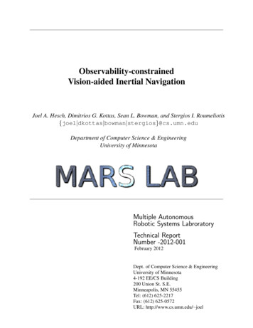
(a)(b)Figure 1: (a) Camera-IMU trajectory and 3D features. (b) Error and 3σ bounds for the rotation about the gravityvector, plotted for a single run. Hcam HθG C I q̄ˆG,k k 1 G g 0.HpI bG f̂k k 1 c bG p̂I,k k 1 c G g(26)This is a constraint of the form Au 0, where u is a fixed quantity determined by elements in the nullspace, and Acomprises elements of the measurement Jacobian. We compute the optimal A that satisfies this relationship usingthe solution to (24). After computing the optimal A , we recover the Jacobian asHcam HθG A01:2,1:3 , Hcam HpI A01:2,4:6 , Hcam Hf A01:2,4:6(27)where the subscripts (i:j, m:n) denote the submatrix spanning rows i to j, and columns m to n. After computing themodified measurement Jacobian, we proceed with the filter update as described in Sect. 3.2.5SimulationsWe conducted Monte-Carlo simulations to evaluate the impact of the proposed Observability-Constrained VINS (OCVINS) method on estimator consistency. We compared its performance to the standard VINS (Std-VINS), as well asthe ideal VINS that linearizes about the true state2 . Specifically, we computed the Root Mean Squared Error (RMSE)and Normalized Estimation Error Squared (NEES) over 100 trials in which the camera-IMU platform traversed acircular trajectory of radius 5 m at an average velocity of 60 cm/s.3 The camera observed visual features distributed onthe interior wall of a circumscribing cylinder with radius 6 m and height 2 m (see Fig. 1a). The effect of inconsistencyduring a single run is depicted in Fig. 1b. The error and corresponding 3σ bounds of uncertainty are plotted forthe rotation about the gravity vector. It is clear that the Std-VINS gains spurious information, hence reducing its3σ bounds of uncertainty, while the Ideal-VINS and the OC-VINS do not. The Std-VINS becomes inconsistent onthis run as the orientation errors fall outside of the uncertainty bounds, while both the Ideal-VINS and the OC-VINSremain consistent. Figure 2 displays the RMSE and NEES, in which we observe that the OC-VINS obtains orientationaccuracy and consistency levels similar to the ideal, while significantly outperforming Std-VINS. Similarly, the OCVINS obtains better positioning accuracy compared to Std-VINS.6Experimental ResultsThe proposed OC-VINS has been validated experimentally and compared with Std-VINS. We hereafter provide anoverview of the system implementation, along with a discussion of the experimental results.6.1Implementation RemarksThe image processing is separated into two components: one for extracting and tracking short-term opportunisticfeatures (OFs), and one for extracting persistent features (PFs) to use in SLAM.2 Since3 Thethe ideal VINS has access to the true state, it is not realizable in practice, but we include it here as a baseline comparison.camera had 45 deg field of view, with σ px 1px, while the IMU was modeled with MEMS quality sensors.TR-2012-0018

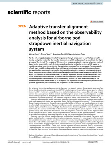
(a)(b)(c)(d)Figure 2: The RMSE and NEES errors for position and orientation plotted for all three filters, averaged per time stepover 100 Monte Carlo trials.OFs are extracted from images using the Shi-Tomasi corner detector [30]. After acquiring image k, it is insertedinto a sliding window buffer of m images, {k m 1, k m 2, . . . , k}. We then extract features from the first imagein the window and track them pairwise through the window using the KLT tracking algorithm [18]. To remove outliersfrom the resulting tracks, we use a two-point algorithm to find the essential matrix between successive frames. Giventhe filter’s estimated rotation between image i and j, i q̄ˆ j , we estimate the essential matrix from only two featurecorrespondences. This approach is more robust than the traditional five-point algorithm [26] because it provides twosolutions for the essential matrix rather than up to ten, and as it requires only two data points, it reaches a consensuswith fewer hypotheses when used in a RANSAC framework.The PFs are extracted using SIFT descriptors [17]. To identify global features observed from several differentimages, we first utilize a vocabulary tree (VT) structure for image matching [27]. Specifically, for an image taken attime k, the VT is used to select which image(s) taken at times 1, 2, . . . , k 1 correspond to the same physical scene.Among those images that the VT reports as matching, the SIFT descriptors from each are compared to those fromimage k to create tentative feature correspondences. The epipolar constraint is then enforced using RANSAC andNister’s five-point algorithm [26] to eliminate outliers. It is important to note that the images used to construct the VT(offline) are not taken along our experimental trajectory, but rather are randomly selected from a set of representativeimages.At every time step, the robot poses corresponding to the last m images are kept in the state vector, as describedin [28]. Upon the ending of the processing of a new image, all the OFs that first appeared at the oldest augmentedrobot pose, are processed following the MSC-KF approach, as discussed earlier. The frequency at which new PFs areinitialized into the map is a scalable option which can be tuned according to the available computational resources,while PF updates occur at any reobservation of initialized features.6.2Experimental EvaluationThe experimental evaluation was performed with an Ascending Technologies Pelican quadrotor equipped with aPointGrey Chameleon camera, a Navchip IMU and a VersaLogic Core 2 Duo single board computer. For the purposes of this experiment, the onboard computing platform was used only for measurement logging and the quadrotorplatform was simply carried along the trajectory. Note that the computational and sensing equipment does not exceedTR-2012-0019

(a)(b)(c)Figure 3: The estimated 3D trajectory over the three traversals of the two floors of the building, along with theestimated positions of the mapped landmarks. (a) projection on the x and y axis, (b) projection on the y and z axis, (c)3D view of the overall trajectory and estimated featuresthe weight or power limits of the quadrotor and it is still capable of flight. The platform traveled a total distance of172.5 meters over 2 floors at the Walter Library at University of Minnesota. IMU signals were sampled at a frequencyof 100Hz while camera images were acquired at 7.5Hz. The trajectory traversed in our experiment consisted of threepasses over a loop that spanned two floors, so three loop-closure events occurred. The quadrotor was returned to itsstarting location at the end of the trajectory, to provide a quantitative characterization of the achieved accuracy.Opportunistic features were tracked using a window of m 10 images. Every m camera frames, up to 30 featuresfrom all available PFs are initialized and the state vector is augmented with their 3D coordinates. The process ofinitializing (see Appendix 1) is continued until the occurrence of the first loop closure; from that point, no new PFsare considered and the filter relies upon the re-observation of previously initialized PFs and the processing of OFs.For both the Std-VINS and the OC-VINS, the final position error was approximately 34 cm, which is less than0.2% of the total distance traveled (see Fig. 3). However, the estimated covariances from the Std-VINS are smallerthan those from the OC-VINS (see Fig. 4). Furthermore, uncertainty estimates from the Std-VINS decreased indirections that are unobservable (i.e., rotations about the gravity vector); this violates the observability properties ofthe system and demonstrates that spurious

extensively validated with simulation trials and real-world experimentation. 1 Introduction A Vision-aided Inertial Navigation System (VINS) fuses data from a camera and an Inertial Measurement Unit (IMU) to track the six-degrees-of-freedom (d.o.f.) position and orientation (pose) of a sensing platform. This sensor pair is