Transcription
DAAAM INTERNATIONAL SCIENTIFIC BOOK 2015pp. 001-016Chapter 01ADVANCED JOB SHOP SCHEDULING METHODSBUCHMEISTER, B. & PALCIC, I.Abstract: Scheduling is a decision-making process used on a regular basis in manymanufacturing and service industries. It plays an important role in shop floor planning.Job shop is one of the most popular generalized production systems. A schedule showsthe planned time when the processing of a specific job will start and will be completedon each machine that the job requires. Schedule is a timetable for both jobs andmachines. Complex and mathematically involved scheduling methods requiresubstantial and extensive knowledge. Since job shop scheduling problems fall mostlyinto the class of NP-hard problems, they are among the most difficult to formulate andsolve. In the chapter, a selection of advanced job shop scheduling methods isrepresented: filtered beam search, constraint-guided heuristic search and geneticalgorithms, all demonstrated with simple examples.Key words: job shop, scheduling, filtered beam search, constraint-guided heuristicsearch, genetic algorithmsAuthors data: Full. Prof. Dr. Sc. Buchmeister, B[orut]; Assoc. Prof. Dr. Sc. Palcic,I[ztok], University of Maribor, Faculty of Mechanical Engineering, ProductionEngineering Institute, Smetanova 17, 2000 Maribor, Slovenia, European Union,borut.buchmeister@um.si, iztok.palcic@um.siThis Publication has to be referred as: Buchmeister, B[orut] & Palcic, I[ztok](2015). Advanced Job Shop Scheduling Methods, Chapter 01 in DAAAM InternationalScientific Book 2015, pp.001-016, B. Katalinic (Ed.), Published by DAAAMInternational, ISBN 978-3-902734-05-1, ISSN 1726-9687, Vienna, AustriaDOI: 10.2507/daaam.scibook.2015.01
Buchmeister, B. & Palcic, I.: Advanced Job Shop Scheduling Methods1. IntroductionOn the market, which is shaped by increasingly more demanding customers, therising number of providers and the competitiveness between them, and right businessand production strategy are the deciding factors of a company’s success (Baesler et al.,2015). It is not enough only to keep up with the others. Today, success representssustainability in introducing new standards and orientation toward the customer, to thequality and price of products, to flexibility, agility and promptness, to economising inresources and protection of the environment (Huang, 2010). There are an increasingnumber of companies, which produce mostly with a job shop system for a knowncustomer. With competitive cost calculation and appropriate product quality, time isbecoming the most important factor of business success. This is especially noticeablein job shop production, where adaptability and shortening of flow times decide on thebusiness success or failure of the company (Buchmeister et al., 2004).Scheduling is as old as humankind is. It is about time and some optimisation. It isan act of defining priority or arranging activities to meet certain requirements,constraints or objectives. Time is always a major constraint. People schedule theiractivities so that jobs could be accomplished within the available time. Time to get up,time to work, to play, to sleep Time is a limiting unrecoverable resource and wemust schedule our activities to utilise this limited resource in an optimum manner.As the industrialized world develops, more and more resources are becoming critical.Machines, workers and facilities are now thought of as resources in production orservice activities. Scheduling these leads to increased efficiency, utilization andprofitability for the company (Yagmahan & Yenisey, 2009).We have to think about time all the time. We trade time for money. Efficient useof time is namely one of the greatest indicators of competitiveness.2. Role and impact of schedulingScheduling is a decision-making process used on a regular basis in manymanufacturing and service industries. These forms of decision-making play animportant role in procurement and production, in transportation and distribution, andin information processing and communication (Blazewicz et al., 2007). The schedulingfunctions in a company rely on mathematical techniques and heuristic methods toallocate limited resources to the activities that have to be done. This allocation ofresources has to be done in such a way that the company optimizes its objectives andachieves its goals. Resources may be machines in a workshop, crews at a constructionsite, or processing units in a computing environment. Activities may be operations ina workshop, stages in a construction project, or computer programs that have to beexecuted. Each activity may have a priority level, an earliest possible starting time anda due date. Objectives can take many different forms, such as minimizing the time tocomplete all activities, minimizing the number of activities that are completed after thecommitted due dates, and so on (Singh, 2014).Within scheduling in manufacturing in the chapter, a generic manufacturingenvironment and the role of its scheduling function will be described. Orders that are
DAAAM INTERNATIONAL SCIENTIFIC BOOK 2015pp. 001-016Chapter 01released in a manufacturing setting have to be translated into jobs with associated duedates. These jobs often have to be processed on the machines in a work-station in agiven order or sequence. The processing of jobs may sometimes be delayed if certainmachines are busy. Preemptions may occur when high priority jobs are released whichhave to be processed at once. Unexpected events on the shop-floor, such as machinebreakdowns or longer-than-expected processing times, also have to be taken intoaccount, since they may have a major impact on the schedules. Developing, in such anenvironment, a detailed schedule of the jobs to be performed helps maintain efficiencyand control of operations (Kaban et al., 2012).Fig. 1. Information flow diagram in a manufacturing system (Pinedo, 2005)
Buchmeister, B. & Palcic, I.: Advanced Job Shop Scheduling MethodsThe scheduling process also interacts with the production planning process, whichhandles medium-term to long-term planning for the entire organization. This processintends to optimize the firm’s overall product mix and long-term resource allocationbased on inventory levels, demand forecasts and resource requirements (Velaga, 2013).Decisions made at this higher planning level may impact the more detailed schedulingprocess directly. Fig. 1 shows the information flow in a manufacturing system.3. Advanced scheduling methods3.1 Filtered beam searchThis method is based on the ideas of branch and bound. Enumerative branch andbound methods are currently the most widely used methods for obtaining optimalsolutions to "NP-hard" scheduling problems. The main disadvantage of branch andbound is that it is usually extremely time consuming, because the number of nodes onemust consider is very large (Fig. 2).Fig. 2. Schematic representation of Filtered Beam SearchConsider, for example, a single machine problem with n jobs. Assume that foreach node at level k, jobs have been selected for the first k positions. There is a singlenode at level 0, with n branches emanating from it to n nodes at level 1. Each node atlevel 1 branches out into n–1 nodes at level 2, resulting in a total of n.(n–1) nodes atlevel 2. At level k, there are n!/(n–k)! nodes. At the bottom level, level n, there are n!nodes. Branch and bound method attempts to eliminate a node by determining a lowerbound on the objective for all partial schedules that sprout out of that node. If the lowerbound is higher than the value of the objective under a known schedule, then the nodemay be eliminated and its offspring disregarded. If one could obtain a reasonably goodschedule through some clever heuristic before going through the branch and boundprocedure, then it might be possible to eliminate many nodes. Even after theseeliminations, there are usually still too many nodes to be evaluated. The mainadvantage of branch and bound is that, after evaluating all nodes, the final solution isknown with certainty to be optimal (Tasic et al., 2007).
DAAAM INTERNATIONAL SCIENTIFIC BOOK 2015pp. 001-016Chapter 01Filtered beam search is an adaptation of branch and bound in which not all nodesat any given level are evaluated. Only the most promising nodes at level k are selectedas nodes to branch from. The remaining nodes at that level are discarded permanently.The number of nodes retained is called the beam width of the search. The evaluationprocess that determines which nodes are the promising ones is a crucial component ofthis method. Evaluating each node carefully, to obtain an estimate for the potential ofits offspring, is time consuming. There is a trade-off here: a crude prediction is quickbut may lead to discarding good solutions, whereas a more thorough evaluation maybe prohibitively time consuming. Here is where the filter comes in. For all the nodesgenerated at level k, a crude prediction is done. Based on the outcome of these crudepredictions, a number of nodes are selected for a thorough evaluation, and theremaining nodes are discarded permanently. The number of nodes selected for athorough evaluation is referred to as the filter width. Based on the outcome of thecareful evaluation of all nodes that pass the filter, a subset of these nodes (the numberbeing equal to the beam width, which, therefore, cannot be greater than the filter width)is selected, from which further branches will be generated.Example 1: Consider the instance of 1 wj Tj (using notation α β γ). Theobjective is to minimize the sum of the weighted tardinesses. Table 1 contains the basicdata (all jobs are available at time zero; due dates are extremely low to expose theobjective function).Job j123pj101013dj421wj14121Tab. 1. Data for four jobs and notation441212j – job numberpj – processing time of jobdj – due date of jobwj – weight of jobBecause the number of jobs is rather small, only one type of prediction is madefor the nodes at any particular level. No filtering mechanism is used. The beam widthis chosen to be 2, which implies that at each level only two nodes are retained. Theprediction at a node is made by scheduling the unscheduled jobs according to the ATC(Apparent Tardiness Cost) rule. With the due-date range factor:R d max d minĈmax(1)R 11/37 and the due-date tightness factor: 1 dCˆ(2)maxτ 32/37, the look-ahead parameter k, estimated by the following equations:k 4.5 R, R 0.5k 6 2 R, R 0.5is chosen to be 5.(3)
Buchmeister, B. & Palcic, I.: Advanced Job Shop Scheduling MethodsA branch and bound tree is constructed with the assumption that the sequence isdeveloped, starting from t 0. So, at the jth level of the tree jobs are put into the jthposition. At the level 1 of the tree, there are four nodes: (1,*,*,*), (2,*,*,*), (3,*,*,*)and (4,*,*,*), see Fig. 3. Using the ATC rule to the remaining jobs at each one of fournodes results in four sequences: (1,4,2,3), (2,4,1,3), (3,4,1,2) and (4,1,2,3) withobjective values 408, 436, 814 and 440. Because the beam width is 2, only the first twonodes are retained.Each of these two nodes leads to three nodes at level 2. Node (1,*,*,*) leads tonodes (1,2,*,*), (1,3,*,*) and (1,4,*,*), and node (2,*,*,*) leads to nodes (2,1,*,*),(2,3,*,*) and (2,4,*,*). Applying the ATC rule to the remaining two jobs in each oneof the six nodes at level 2 results in nodes (1,4,*,*) and (2,4,*,*) being retained and theremaining four being discarded.Two nodes at level 2 lead to four nodes at level 3 (the last level), (1,4,3,2),(1,4,2,3), (2,4,1,3) and (2,4,3,1). Of these four sequences, sequence (1,4,2,3) is the bestwith a total weighted tardiness equal to 408. This sequence is optimal.Fig. 3. Beam search applied to 1 wjTj3.2 Constraint-guided heuristic searchIn many real-world situations, there is not really an objective. Rather it is requiredonly to generate a feasible schedule that satisfies various constraints and rules. Oneapproach for generating schedules in these situations is referred to in the literature(Pinedo, 2005) as constraint-guided search. This approach has been very popularamong computer scientists and artificial intelligence experts.Constraint-guided search may be described best through an example. Consider anumber of not necessarily identical machines in parallel. A job has to be processed only
DAAAM INTERNATIONAL SCIENTIFIC BOOK 2015pp. 001-016Chapter 01on the one of the machines; for each job there may be a feasible set of machines Mj tochoose from. Job j requires a processing time pj 1, j 1, , n and has release date rjand the due date dj. The goal is to find a feasible schedule in which all jobs areprocessed within their respective time windows. In this case the optimal schedule hasan objective of value 0 (perfect feasibility).Constraint-guided search may operate according to the following rules. Jobs arescheduled one at a time. When a job is scheduled, it is assigned to a specific time sloton a specific machine, which is still free. At the each iteration, an unassigned job isselected according to a set of job rules that have been arranged in some priority. Thejob rules specify whether the particular job actually can be processed on a givenmachine.The jobs can be ordered according to their criticality or flexibility; the job withthe least flexibility is the most critical and has the highest priority. The flexibility of ajob can be measured in several ways (flexibility in time – slack time, flexibility withregard to the number of appropriate machines, etc.).The machines also can be ordered in such a way that the machine with the leastflexibility has the highest priority (the flexibility of a machine, measured by the numberof jobs that can be processed on the machine).An important concept in constraint-guided search is constraint propagation. Theassignment of a particular job to a given time slot on a given machine has implicationswith regard to the assignment of other jobs on the given machine and on othermachines. These implications may point to the violation of hard constraints and mayindicate that the associated part of the search space can be disregarded.Example 2: Consider the problem P3 rj, pj 1, Mj Uj. Uj 1, if Cj dj,otherwise Uj 0. We have three machines and nine jobs. The processing times, releasedates, and due dates of the job are presented in Table 2. If the processing time of a jobon a machine is infinity ( ), then the job cannot be processed on that machine. Thegoal is to find a feasible schedule with all jobs completed on time (Σ Uj 0).Job j12p1j1 p2j11p3j11rj11dj32Tab. 2. Data for nine jobs31 014 110251110167 1 01113811 13911123There are nine timeslots and three on each machine. Each job has its own timewindow, which represents a set of constraints. For each job, a flexibility factor Фj canbe calculated. In this example: Фj is the number of timeslots to which a job may beassigned on various machines. The flexibility factor Фj of job j is presented in Table 3.Instead of the flexibility of a machine, the flexibility of a timeslot on a machine isdetermined. It is defined as the number of jobs that can be processed during thetimeslot. The flexibility factor Ф(i,l) of job timeslot (i, l ) is presented in Table 4.
Buchmeister, B. & Palcic, I.: Advanced Job Shop Scheduling MethodsJob j1234Φj4314Tab. 3. Flexibility factor of nine jobs53Machine11122Timeslot (1, 1) (1, 2) (1, 3) (2, 1) (2, 2)Φ(i,l)22234Tab. 4. Flexibility factor of job timeslot617223(2, 3) (3, 1)32849333(3, 2) (3, 3)43Sequence of jobs in increasing flexibility results in: 3, 6, 7, 2, 5, 9, 1, 8, 4.Priorities of the timeslots may result in the sequence (1, 3), (3, 1), (1, 1), (1, 2), (2, 1),(2, 3), (3, 3), (3, 2), (2, 2).Job 3 is selected first. It is checked to determine whether it is allowed to beprocessed in the timeslot (1, 3). It is not (too late). The next timeslot is tried (3, 1) – noton 3rd machine, and so on, until a timeslot is found during which it is allowed to beprocessed. Job 3 is then assigned to slot (1, 1). Job 6 is considered in the same mannerand assigned to slot (2, 1). Continuing in this manner results in the followingassignment – see Table 5. All the constraints are fulfilled.Timeslot (1, 1) (1, 2) (1, 3) (2, 1)Job3296Tab. 5. Assignment of jobs to timeslots(2, 2)8(2, 3)1(3, 1)5(3, 2)4(3, 3)7After a job has been assigned, the flexibility factors of the remaining jobs to beassigned and the remaining timeslots available may change. It would have beenpossible to reorder the remaining jobs, as well as the remaining timeslots, based on thenew flexibility factors. In the example above this was not done.Constraint-guided search does not always yield a feasible solution after the firstpass. It may occur that when the last job has to be assigned, no feasible assignment ispossible. In this case, the method has to rely on a postprocessing procedure, which,through pairwise interchanges, attempts to construct a feasible solution.3.3 Genetic algorithmsGenetic algorithms (GA) are an optimization methodology based on a directanalogy to Darwinian natural selection and mutations in biological reproduction. Inprinciple, genetic algorithms encode a parallel search through concept space, with eachprocess attempting coarse-grain hill climbing. Instances of a concept correspond toindividuals of a species. Induced changes and recombinations of these concepts aretested against an evaluation function to see which ones will survive to the nextgeneration (Gao et al., 2007). The use of genetic algorithms (Fig. 4) requires fivecomponents:1. A way of encoding solutions to the problem – fixed length string of symbols.2. An evaluation function that returns a rating for each solution.
DAAAM INTERNATIONAL SCIENTIFIC BOOK 2015pp. 001-016Chapter 013. A way of initializing the population of solutions.4. Operators that may be applied to parents when they reproduce to alter their geneticcomposition such as crossover (i.e., exchanging a randomly selected segment betweenparents), mutation (i.e., gene modification), and other domain specific operators.5. Parameter setting for the algorithm, the operators, and so forth.Fig. 4. Structure of a simple genetic algorithmTwo basic encoding approaches, direct and indirect, are applicable. The directapproach encodes a job shop schedule as a chromosome and the genetic operators areused to evolve these chromosomes into better schedules. In the indirect approach, asequence of decision preferences is encoded into the chromosome, for examplescheduling rules for job assignments, and the genetic operators are applied to improvethe ordering of the various preferences. A job shop schedule is then generated from thesequence of preferences (Nagano et al., 2008).A number of approaches have been utilized in the application of geneticalgorithms (GA) to scheduling problems:1. Genetic algorithms with blind recombination operators have been utilized in jobshop scheduling. Their emphasis on relative ordering schema, absolute orderingschema, cycles, and edges in the offsprings will arise differences in such blindrecombination operators.2. Sequencing problems have been also addressed by the mapping of their constraintsto a Boolean satisfiability problem using partial payoff schemes. This scheme hasproduced good results for very simple problems.3. Heuristic genetic algorithms have been applied to job shop scheduling. In thesegenetic schemes, problem specific heuristics are incorporated in the recombinationoperators (such as optimization operators based).Example 3: A simple genetic algorithm is used to treat the job shop problem. Thisalgorithm was developed independently, without regard for the work of otherresearchers (Lestan et al., 2009). The intention was to make a simple algorithm, whichwill try to find the schedule with the smallest makespan. Only genetic operations areused in order to achieve this. It is possible to schedule a various number of jobs, but
Buchmeister, B. & Palcic, I.: Advanced Job Shop Scheduling Methodsneither release times nor due dates are considered. Only selection and permutation areused as genetic operations. The algorithm uses random moves to search for the optimalschedule in the solution space, which means that the solution is obtained without thehelp of heuristic methods.How to encode solutions to chromosomes to ensure feasible solutions is a keyissue for genetic algorithms. In our algorithm, the preference list-based representationis used. In this encoding method, the operations are arranged in a certain order. Itdepends on this order, how the operations will be processed on the machines. It is veryimportant, that the precedence constrains of operations of individual jobs areconsidered. This means, that the sequence of operations of a job must stay intact alsoin the encoded solution. How the encoding works is shown on a simple example. Table6 shows a 3 3 instance; 3 jobs (9 operations) must be scheduled on 3 machines (M1,M2, M3) to achieve the smallest possible makespan.Processing timesJobsOperations123J129789J2439028J3918574Tab. 6. Data for a 3 3 instanceProcessing orderOperations123machine M1machine M2 machine M3machine M1machine M3 machine M2machine M2machine M1 machine M3From the Table 6 it is possible to write the operation sequence for each job:J1 (J1 M1 29) (J1 M2 78) (J1 M3 9)J2 (J2 M1 43) (J2 M3 90) (J2 M2 28)J3 (J3 M2 91) (J3 M1 85) (J3 M3 74)Job J1 must first be processed on machine M1 for 29 time units. After that onmachine M2 for 78 units and the last is machine M3 for 9 units. Similar goes for theother two jobs. The schedule for this instance is encoded into a string, where theposition of the operation in the string plays an important role. Operations are orderedwith the help of a randomizer. Therefore, it is important to use a reliable randomizer.String making in our case looks like this:a) A list of first operations of all jobs has been made.((J1 M1 29) (J2 M1 43) (J3 M2 91))b) From the list of first operations, one operation is chosen randomly; let’s say (J2 M143). This operation is the first operation in the string. The operation is taken from thecorresponding job and inserted into the string.J1 (J1 M1 29) (J1 M2 78) (J1 M3 9)J2 (J2 M3 90) (J2 M2 28)J3 (J3 M2 91) (J3 M1 85) (J3 M3 74)String:((J2 M1 43))
DAAAM INTERNATIONAL SCIENTIFIC BOOK 2015pp. 001-016Chapter 01c) Again, a list of first operations of all the jobs is made and an operation is randomlyselected from the list; let’s say (J1 M1 29). This operation is taken from thecorresponding job and inserted as second operation in the string.J1 (J1 M2 78) (J1 M3 9)J2 (J2 M3 90) (J2 M2 28)J3 (J3 M2 91) (J3 M1 85) (J3 M3 74)String:((J2 M1 43) (J1 M1 29))d) The procedure is repeated until all the operations from the jobs are transferred intothe string.If the procedure, described above, would be continued until the end, the stringcould look like this:((J2 M1 43) (J1 M1 29) (J1 M2 78) (J3 M2 91) (J2 M3 90)(J3 M1 85) (J2 M2 28) (J1 M3 9) (J3 M3 74))This string will be used later on for demonstrations. A closer look at the stringreveals that the precedence constrains have been considered during the making of thestring. Job operations in the string still have the same processing order, but now theyare mixed together. Why this is so important is explained below.Because the string making is left to coincidence, it is possible to make manyversatile strings (organisms) which are necessary for the initial population.Only feasible strings represent a solution to our problem and therefore it is veryimportant that feasibility is maintained throughout the searching process. Because inour case the goal lies in the time optimization of schedules, we are interested in themakespan. Besides the makespan, we are interested also in the processing order on themachines. The Gantt chart (string evaluation) is done step by step with addingoperations one after another. In our case, the operations are added directly from thestring, from the left side to the right side. The operations, which are at the beginning ofthe string, have a higher processing priority than those at the end. This means, that theGantt chart and the makespan depend only upon the order in the string. That is why itis so important, that the operation order in the string is according to the precedenceconstrains. Otherwise, the evaluation would give a false value. The Gantt chart for ourstring is shown in Fig. 5.Fig. 5. Gantt chart for the 3 3 instance
Buchmeister, B. & Palcic, I.: Advanced Job Shop Scheduling MethodsString:((J2 M1 43) (J1 M1 29) (J1 M2 78) (J3 M2 91) (J2 M3 90)(J3 M1 85) (J2 M2 28) (J1 M3 9) (J3 M3 74))Because the use of graphic Gantt charts in programming would be annoying,Gantt charts in numerical form are used. These charts are not as synoptic as graphical,but it is possible to comprehend all the important data from them. The Gantt chart inFig. 4 looks in numerical form like this:M1 (0 J2 43) (43 J1 72) (241 J3 326)M2 (72 J1 150) (150 J3 241) (241 J2 269)M3 (43 J2 133) (150 J1 159) (326 J3 400)Genetic operations are the driving force in genetic algorithms. Which operationsare reasonable to use for solving a certain problem depends on the encoding method.The only genetic operation, which is independent from encoding, is selection. Selectionis the most simple of all genetic operations. In our algorithm, the tournament selectionis used. Its purpose is to maintain the core of good solutions intact. This is done withtransferring good solutions from one generation to the next one. Because selection doesnot change the organism (string), we have no problem with maintaining feasibility,which is not the case in all other genetic operations. The use of the crossover operationcan be problematical in some cases. The crossover operation often produces infeasibleoffspring, which are difficult to repair.The only genetic operation besides selection, which is used in our algorithm, ispermutation. The permutation is based on switching operations inside the organism.The organism, which will be permutated, is chosen with the selection. When executingthe permutation it is necessary to consider the precedence constrains. The permutationprocedure is described and shown on our string from Table 6:a) A random operation is chosen from the string; let’s say (J2 M1 43).String:((J2 M1 43) (J1 M1 29) (J1 M2 78) (J3 M2 91) (J2 M3 90)(J3 M1 85) (J2 M2 28) (J1 M3 9) (J3 M3 74))b) The left and the right border for the chosen operation have to be defined. Becausethe chosen operation belongs to job J2, it is necessary to search for the first operation,left and right of the chosen operation, which belongs to job J2. If the operation doesnot exist, the border is represented by the end or the beginning of the string. In ourcase, the right border is represented by the operation (J2 M3 90) and the left border ispresented by the beginning of the string. In the string, the space between the borders ismarked with square brackets.String:([(J2 M1 43) (J1 M1 29) (J1 M2 78) (J3 M2 91)] (J2 M3 90)(J3 M1 85) (J2 M2 28) (J1 M3 9) (J3 M3 74))
DAAAM INTERNATIONAL SCIENTIFIC BOOK 2015pp. 001-016Chapter 01c) A random position between the brackets is chosen where the operation (J2 M1 43)is inserted; let us say in front of (J1 M2 78).String:((J1 M1 29) (J2 M1 43) (J1 M2 78) (J3 M2 91) (J2 M3 90)(J3 M1 85) (J2 M2 28) (J1 M3 9) (J3 M3 74))This procedure randomly changes the chosen organism, which also changes thesolution, which the organism represents. Because there is often necessary to switchmore than one operation in the organism, it is possible to repeat the whole procedureover and over.Evolution parameters are parameters, which influence the searching procedure ofthe genetic algorithm. If we want to obtain good solutions, the parameters have to beset wisely. These parameters are: selection pressure, population size, amount of change, made by genetic operation, share of individual genetic operations in the next generation, number of generations (stopping criterion), number of independent civilizations.The selection pressure defines what kind of solutions will be used in geneticoperations. If the selection pressure is high, then only the best solutions will get thechance. If it is low, then also worse solutions are used. The higher the selectionpressure, the higher the possibility that the search will end up in a local optimum. If itis too low, the search procedure examines insignificant solutions, which protracts thewhole search.When an organism is being modified, it is necessary to specify how much thegenetic operation will change the organism. It is recommended that small and largechanges are made to the organisms. This assures versatility in the population.Each genetic operation must make a certain amount of organisms for the nextgeneration. At least 10 % of the next population has to be made with selection(Brezocnik, 2000), so that the core of good solutions is maintained. All the otherorganisms are created with other genetic operations.If the number of generations is multiplied with the size of the population, we getthe number of organisms, which have been examined during the search. When solvingcomplex problems, the number of organisms is greater than in easier cases. Thequestion is, should the search be executed with a small population and a lot ofgenerations or opposite. In most cases, a compromise is the best choice.Because the search with genetic algorithms bases on random events, it is notnecessary that good solutions are obtained in every civilization. In most cases, thesearch stops in a local optimum. That is why it is necessary to execute multiple searchesfor a given problem.The algorithm was tested on the benchmark 10 10 instance (see the results inTable 7 for the data in Table 8), which was proposed by Fisher and Thompson (1963).
Buchmeister, B. & Palcic, I.: Advanced Job Shop Scheduling MethodsRows contain
Abstract: Scheduling is a decision-making process used on a regular basis in many manufacturing and service industries. It plays an important role in shop floor planning. Job shop is one of the most popular generalized production systems. A schedule shows the planned time when the processing of a specific job will start and will be completed