WIXLIB

Data Visualization (DSC 530/CIS 602-01)Trees & Geospatial DataDr. David KoopD. Koop, DSC 530, Spring 2016

Arrange TablesArrange TablesExpress ValuesSeparate, Order, Align RegionsSeparateOrderAlign1 KeyList2 KeysMatrix3 KeysVolumeMany KeysRecursive SubdivisionAxis OrientationRectilinearParallelRadialLayout DensityDenseSpace-Filling[Munzner (ill. Maguire), 2014]D. Koop, DSC 530, Spring 20162

SPLOMs and Parallel CoordinatesScatterplot MatrixParallel zner (ill. Maguire), 2014]D. Koop, DSC 530, Spring 20163

The main difficulty of directly applying parallel coordntheirandmethod.extents Moreof clusters withof varyingtranslulargebandsdata setsis that thelevel of clutter present in the visuable, it is difficult toreduces the amount of useful information one can perceOverdraw in Parallelexample, Coordinatesthe display of a mass of overlapping lines precque for hierarchicalperception of relative densities present in the data set (serallelCoordinatese-map idea[24] by2: Parallelcoo2). Our approach reduces the amountFigureof clutterby imposinssimilarity measure.a 5-dimensional dataustering results, andover-plotting precludmilarity value.tions or anomalies.found in the abovedata at multiple resarchical organizationdering limitation ofof the data at differeechniques. We alsodynamically navigatitter. However, ratherdetail in the followinines, we use data agusters, and show theof varying translu-4 OverviewdinatesParallel coordinates of Detroitset: a 7-display of a Remote SensingFigurehomicide2: Paralleldatacoordinates[Fua et al.,1999]Exploratorydataanalnal data set with 13 records.a 5-dimensionalNotice that therearesetinversedatawith 16,384 records. Note eptionofanydatatrends,Koop, DSC 530, Spring 2016

Arrange Networks and TreesArrange Networks and TreesNode–Link DiagramsConnection MarksNETWORKSTREESAdjacency MatrixDerived TableNETWORKSTREESEnclosureContainment MarksNETWORKSTREES[Munzner (ill. Maguire), 2014]D. Koop, DSC 530, Spring 20165

Web Sites as Graphs (amazon.com)[M. Salathe, 2006]D. Koop, DSC 530, Spring 20166

Arc Diagram[D. Eppstein, 2013]D. Koop, DSC 530, Spring 20167

Force-Directed Layout Nodes push away from each otherbut edges are springs that pull themtogether Weakness: nondeterminism,algorithm may produce differenceresults each time it runs[M. Bostock, 2012]D. Koop, DSC 530, Spring 20168

sfdp[Hu, 2005]D. Koop, DSC 530, Spring 20169

Adjacency Matrices[McGuffin]D. Koop, DSC 530, Spring 201610

Node-Link or Adjacency Matrix? Empirical study: For most tasks, node-link is better for small graphsand adjacency better for large graphs Multi-link paths are hard with adjacency matrices Immediate connectivity or neighbors are ok, estimating size (nodes& edges also ok) People tend to be more familiar with node-link diagrams Link density is a problem with node-link but not with adjacencymatricesD. Koop, DSC 530, Spring 201611

Assignment 2 www.cis.umassd.edu/ dkoop/dsc530/assignment2.html Use D3! 2016 Campaign Finance Data- Changes from mid- to end-2015- Including SuperPAC receipts- Extra Credit: Transitions Cheating Questions?D. Koop, DSC 530, Spring 201612

Arrange Networks and TreesArrange Networks and TreesNode–Link DiagramsConnection MarksNETWORKSTREESAdjacency MatrixDerived TableNETWORKSTREESEnclosureContainment MarksNETWORKSTREES[Munzner (ill. Maguire), 2014]D. Koop, DSC 530, Spring 201613

Trees Trees are directed acyclic graphs- each edge has a direction: the origin is the parent, the destinationis the child- cannot get back to a node after leaving it A tree has a root (every other node hangs off it) Can consider enclosure in trees using parent-child relationshipsD. Koop, DSC 530, Spring 201614

fair comparison of them. Space-efficiency might be described in termsof area, aspect ratio, label size, or other measures. However, there is noaccepted standard set of metrics for evaluating the space-efficiency oftree representations, and it is unclear what approach would be generalenough to be applied to all the forms in Figure 1.article shows ththat there is moTreemaps arbecause they hwhat we call acated more or lpopulation, or ntitioning can beindeed desirablFigure 2 showstioning of area,borders of nodeFurthermorethe relative sizeeffect is that laare more intererelative sizes, aeach leaf nodeof nodes. (Althaugmented to nterms of label sable, but evenbels, suggestinrepresentation mClearly, it wtinguish2010]the fou[McGuffin and Robert,tive scalabilityFig.Spring1. Several15D. Koop, DSC 530,2016basic kinds of tree representations, here each showing metric of spaceTree Visualizations

Node-Link DiagramIEEE TRANSACTIONS ON SOFTWARE ENGINEERING, VOL. SE-7, NO. 2, MARCH 1981 Trees are graphs223Tidier Drawings of TreesEDWARD M. REINGOLD AND JOHN S. TILFORD but we have more structure Horizontal or verticalAbstract-Various algorithms have been proposed for producing tidydrawings of trees-drawings that are aesthetically pleasing and use minimum drawing space. We show that these algorithms contain somedifficulties that lead to aesthetically unpleasing, wider than necessarydrawings. We then present a new algorithm with comparable time andstorage requirements that produces tidier drawings. Generalizationsto forests and m-ary trees are discussed, as are some problems in discretization when alphanumeric output devices are used. Idea 1: partition space for eachnode via recursion Idea 2: “Tidy” Drawing- Wetherell & Shannon: Don’t wastespace (overlapping parent nodesINTRODUCTIONis ok)IN a recent article [6], Wetherell and Shannon presented algoIndex Terns-Data structures, trees, tree structures.rithms for producing "tidy" drawings of trees-drawingsandspaceTilford:- Reingoldas possible Keepthat use as littlewhile satisfying certainaesthetics. The basic task is the assignment of x and y cosymmetry,looka straightforwardwhichsimilarordinates to eachsubtreesnode of a tree, afterplotting or printing routine generates a drawing of the tree.Wetherell and Shannon give three aesthetics in an attempt todefine a "tidy" drawing of a binary tree.Aesthetic 1: Nodes at the same level of the tree should liealong a straight line, and the straight lines defining the levelsshould be parallel.A left sonAestheticshould be positioned to the left ofD. Koop, DSC530,2:Spring2016Fig. 1. Final positioning of example tree as drawn by Algorithm WS.of the next available position on each level with an arrayNEXT POS, indexed by level, in which each value is set to twoAlg.,ReingoldandTilford,1981]than thegreater [WScoordinateof the lastnodeassigned onthecorresponding level.If a provisional position is less than the next available posi- 16tion on that level, the node is given the next available position,

Reingold-Tilford Algorithm Recurse on left and right subtrees224IEEE TRANSACTIONS ON SOFTWARE ENGINEERING, VOL. SE-7, NO. 2, MARCH 1981 Shift subtree over as long as itdoesn’t overlap Place parent centered above thesubtrees Originally, only binary trees,extended by WalkerFig. 4. A tree and its mirror image positioned by Algorithm WS.Fig. 2. Example tree as drawn by Algorithm TR.[Reingold and Tilford, 1981]D. Koop, DSC 530, Spring 201617

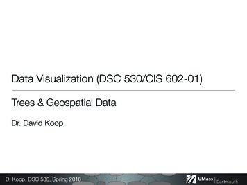
Icicle Plot Line marks Vertical position shows depth Horizontal position shows links andsibling order Scalability: 1 pixel leaves, butharder to label[Bostock, 2011]D. Koop, DSC 530, Spring 201618

Radial Node-Link Use polar coordinates instead of xorwhereDi Fsp ilD la teCo ate ys rAr lor sra sTiysSc meSale caTyp leQuantit RootSScaleeQua ativeS calecnOrdintileScaalealSc lealeLogLinearSScalecaleIScaleMapscaerylequeod appNiHeaHe accnboiFutiD. Koop, DSC 530, Spring 2016teernv roers xtC ertrte Te nvve ited LCo rter rneCoelimphM onv verteD ra taC onG a NCIDSOJrr ntne Eveoinsit tioan siTr raneenT we rsTe rt l d anvaFie hemoc at ScD ata Set ceD ata ourD ataS bleD ataTa ilD taUtDaeSpritDirtySpriteLine hysicsIForceNBoPart dyForceSimuicleSp latioSprring ningForceAAnggregateAri dExpA thresB ve mesioC in rag ticnCo omaryE eCo m pa xpD u p ris reat n os o sseU t ite n ionExtilpressionadded ragan e t tav un ncco istid ivdr eqtofn trag tengfct io Itein s nifst res sioisaDi xp resltE xplte xEmainFnm odIf A alIs rm leLit atch ummuqM axim dsne tM thonomeinimumor erbyM tord eNorangOr ryselectQue ceettePal tteSizeePalelettep aeSha PPalettlortrixaCoM trixrse IMaatrixaSpeMnsDeeaxissStringtsSta rtSo speShapertyPro alettenp atio sent athOri M mathyoxPr ate elue edic abl apaIV IPr alu he eAxisGridLiAxisAxesimatealizLSe To atio eglec olt nE enidpDation Ev ventaEEv ent tTreeeB ven ntSctuilaledeB Tr rNo reindineeEd deS nde gevenDa geSpprite rta ritsDatSpriteteaListDataTdatSeleooltipCoaPanZ ctionConntroloomC trolontrolHove trolListlControlClickControlAnchorControlpeEd IRRendge en erArrRenddereerow ere rTyp rchicalC ctureMergeEdg lusteregraphBetweeLinkD nuEasStpann tPathF siningT sre ein unc gAspIScterp tionSectRPa he ola equatioArBrPa ra du teeaanknce Col yIntll lSerD or erS c us el ableIntateInInterppolatoTr eq hed eMa erpo terp olat ran ue uleoroN tr lsi nc rtio eO um ixIn ato latorP bj be te rnReointectIn rInterpolacta Int ter rpo torng erp pol latoleI ola ato rnte tor rrpolator Benefit: space usage, dAreaLayouOprSequencisetRandomLayoutyout OperatoOperatorL LinkTLa uttionayouttaliza torudTreeLVisu operaIndente reeLayo ckin ayouelaLbrPelealCircle CircgeRoutouttorayEdera erdled AxisLOprltIefilBunabe ereaL bel rdAr lLa eleercke R a d i a L a brodStailte rnceityF iltenibil eF terVis nc Filtioeorista reeerhD eTist ang mod rdap eync de rGr FishR IteeE nco de rnd ndSiz eE co de rnge geap E co deyShpert En nco onLe LeEti noor tio nPrlorist tor tioCoeD is torey D DislshFicafoBi Same layout algorithms work(e.g. Reingold-Tilford)[Bostock, 2012]19

ayoutLayutayoeeLouteTrLay ttedyo uirecLaeDingckramPaeLaylaeTPropreeFertilteEn yEco ncrde odr erDisBifoc FishlIcicndCiAx Intuitive navigationcForDecleCir Reading labels?reeLayRadialTNode Icicle plot in a radial suaD. Koop, DSC 530, Spring ingsisaxSh a p eltro lon ntroCopioltnCTo romGethsMaDacoDLisata[Heer et al., 2012]20

Nested Circles Looks more like cluster diagram,but shows hierarchyTransi TweenEasingColor SizPa Sha Containment shown by the layeringof semi-transparent circlesFunctPara TrP ISSchedSequeTransitioPo ObInterpArr Da Nu MatRec olorsSpaCompGr SimulaSp I DrSpr ParIMa DenStringsJSOC IDDaGraphMDDDat DatEnco ColSh SiPropLabeleSta RadiTextSpLi RectShort LinkDTreeMaDendSpa BetwMaxFloAgglAspecHiera MCommNodeLinIcicRadialTCirclePVisualizPanZHoveAncI Co ContExpClicISc ScLi Ro ScalQuaLog OrdiLayoutIndBundRa Pie AxisLCircleSelectBifoOpeOpeIO SorFishOperOper Gra VisiQuanStackeAxisDat SeVi ToDistoFisTimeSForceDCarte AxAALege LegendQueryFlarDatLegendExprn l ds a osuoem wag vmcm xs and s iml g fi rDirtySDeli Labeling becomes more difficultMatc CompExprNo LiVaRa M MFnXoStriCSAg AvDi Or An BinDate Va IsA IfAritStatsOr IVHe FibonaI IFil PropeDataDraTooltiShaEdgeR I ADataListTreeBuEdg TreeNodeSpritDataSpScaleBi[Bostock, 2012]D. Koop, DSC 530, Spring 201621

Indented Outline Like a filesystem tree Use horizontal position to showdepth, vertical positions showsibling/orderD. Koop, DSC 530, Spring 201622

leLineSprite nsitioner SelectionEvent LegendRangeDataEventDirtySprite ce nsitionInterpolatorClickControl tOr And ExpressionRangeVariance IsASortDatesArraysIfColors EdgeSprite TreeFisheyeTreeFilter ut cciHeapArithmeticDataUtil DataSourceStringUtilDataSprite endrogramLayoutPaletteselect xorwherecountstddevadd eq div ltupdatenotShapePalettesumColorPaletteorderbyfn neq gt lte gteminormaxComparisonisa subandSizePaletteaveragemul iff stStringsDataIcicleTreeLayout emap[Bostock, 2012]click or option-click to descend or ascendSizeD. Koop, DSC 530, Spring 201623

Treemap Containment marks instead of connection marks At each step, orientation of division (horiz/vert) changes Encodes some attribute of the items as the size of the rectangles Not as easy to see the intermediate rectangles Scalability: millions of leaf nodes and links possible Canonical example: Disk inventoryD. Koop, DSC 530, Spring 201624