Transcription
IEEE TRANSACTIONS ON DEPENDABLE AND SECURE COMPUTING,VOL. 8,NO. 1,JANUARY-FEBRUARY 2011147The Geometric EfficientMatching Algorithm for FirewallsDmitry Rovniagin and Avishai Wool, Senior Member, IEEEAbstract—Since firewalls need to filter all the traffic crossing the network perimeter, they should be able to sustain a very highthroughput, or risk becoming a bottleneck. Firewall packet matching can be viewed as a point location problem: Each packet (point)has five fields (dimensions), which need to be checked against every firewall rule in order to find the first matching rule. Thus,algorithms from computational geometry can be applied. In this paper, we consider a classical algorithm that we adapted to the firewalldomain. We call the resulting algorithm “Geometric Efficient Matching” (GEM). The GEM algorithm enjoys a logarithmic matching timeperformance. However, the algorithm’s theoretical worst-case space complexity is Oðn4 Þ for a rule-base with n rules. Because of thisperceived high space complexity, GEM-like algorithms were rejected as impractical by earlier works. Contrary to this conclusion, thispaper shows that GEM is actually an excellent choice. Based on statistics from real firewall rule-bases, we created a Perimeter rulesmodel that generates random, but nonuniform, rule-bases. We evaluated GEM via extensive simulation using the Perimeter rulesmodel. Our simulations show that on such rule-bases, GEM uses near-linear space, and only needs approximately 13 MB of space forrule-bases of 5,000 rules. Moreover, with use of additional space improving heuristics, we have been able to reduce the spacerequirement to 2-3 MB for 5,000 rules. But most importantly, we integrated GEM into the code of the Linux iptables open-sourcefirewall, and tested it on real traffic loads. Our GEM-iptables implementation managed to filter over 30,000 packets-per-second on astandard PC, even with 10,000 rules. Therefore, we believe that GEM is an efficient and practical algorithm for firewall packetmatching.Index Terms—Network communication, network-level security and protection.Ç1INTRODUCTION1.1Motivationfirewall is one of the central technologies allowinghigh-level access control to organization networks.Packet matching in firewalls involves matching on manyfields from the TCP and IP packet header. At least fivefields (protocol number, source and destination IP addresses, and ports) are involved in the decision which ruleapplies to a given packet. With available bandwidthincreasing rapidly, very efficient matching algorithms needto be deployed in modern firewalls to ensure that thefirewall does not become a bottleneck.Modern firewalls all use “first-match” semantics [5], [40],[43]: The firewall rules are numbered from 1 to n, and thefirewall applies the policy (e.g., pass or drop) associatedwith the first rule that matches a given packet. See Fig. 1 foran illustrated example.Firewall packet matching is reminiscent of the wellstudied router packet matching problem. However, there areseveral crucial differences which make the problems quitedifferent. First, unlike firewalls, routers use “longest prefixmatch” semantics. Next, the firewall matching problem is 4Dor 5D, whereas router matching is usually 1D or 2D: A routertypically matches only on IP addresses, and does not lookdeeper, into the TCP or UDP packet headers. Finally, majorTHEfirewall vendors support rules that utilize IP address ranges,in addition to subnets or CIDR blocks1: this is the case forCheck Point and Juniper—the main exception is Cisco thatonly supports individual IP addresses or subnets. Therefore,firewalls require their own special algorithms. The authors are with the School of Electrical Engineering, Tel AvivUniversity, Ramat Aviv 69978, Israel.E-mail: dmitry.rovniagin@gmail.com, yash@acm.org.1.2 Statefull Firewall MatchingMost modern firewalls are stateful. This means that after thefirst packet in a network flow is allowed to cross thefirewall, all subsequent packets belonging to that flow, andespecially the return traffic, is also allowed through thefirewall. This statefulness has two advantages. First, theadministrator does not need to write explicit rules for returntraffic—and such return-traffic rules are inherently insecuresince they rely on source-port filtering (see discussion in[43] and Check Point’s patent [29]). So, stateful firewalls arefundamentally more secure than simpler, stateless, packetfilters. Second, state lookup algorithms are typically simplerand faster than rule-match algorithms; hence, statefulnesspotentially offers important performance advantages.Firewall statefulness is commonly implemented by twoseparate search mechanisms: 1) a slow algorithm thatimplements the “first match” semantics and compares apacket to all the rules and 2) a fast state lookup mechanismthat checks whether a packet belongs to an existing openflow. In many firewalls, the slow algorithm is a naive linearsearch of the rule-base, while the state lookup mechanismuses a hash table or a search tree: This is the case for theManuscript received 24 Dec. 2004; revised 17 May 2006; accepted 21 Apr.2009; published online 22 July 2009.For information on obtaining reprints of this article, please send e-mail to:tdsc@computer.org, and reference IEEECS Log Number TDSC-0184-1204.Digital Object Identifier no. 10.1109/TDSC.2009.28.1. It is possible to convert an arbitrary range of IP addresses into acollection of subnets—however, as many as 62 subnets may be necessary tocover a single IP address range. Thus, there is a great loss of efficiency in theconversion.1545-5971/11/ 26.00 ß 2011 IEEEPublished by the IEEE Computer Society
148IEEE TRANSACTIONS ON DEPENDABLE AND SECURE COMPUTING,VOL. 8,NO. 1,JANUARY-FEBRUARY 2011Fig. 1. Excerpts from a Cisco PIX firewall configuration file, showing two rules. Both rules refer to the TCP protocol. The source in both rules is thesame subnet. The first rule has a single IP address as a destination but a range of destination ports (1-65535), while the second rule has a range ofdestination IP addresses but a single destination port. Note that a TCP packet with source IP 12.20.51.1, destination IP 1.2.3.4, and destination port135 matches both rules, but because of the first match semantics, the first rule’s decision (“permit”) is triggered.open-source firewalls pf [24] and iptables [23]. There arestrong indications that commercial firewalls use linearsearch for the slow rule match as well: e.g., Check Pointrules are translated into an assembly-like macro languagecalled INSPECT [40] with linear semantics, and theINSPECT language is simply translated into bytecode.Moreover, the standard advise for improving firewallperformance, for all vendors, is to place the most popularrules near the top of the rule-base (cf., [14], [7]). This advisedoesn’t make much sense if the firewall rearranges the rulesinto a complex search data structure.Note that a stateful firewall’s two-part design provides itshighest performance on long TCP connections, for which thefast state lookup mechanism handles most of the packets.However, connectionless UDP2 and ICMP traffic, and shortTCP flows, like those produced in extremely high volume byDistributed Denial of Service attacks (cf., [19]), only activatethe “slow” algorithm, making it a significant bottleneck. Ourmain result is that the “slow” algorithm does not need to beslow, even in a software-only implementation running on ageneral-purpose operating system. We show that theGEM algorithm has a matching speed that is comparableto that of the state lookups: In isolation, the algorithmrequired under 1 sec per packet, and our Linux GEMiptables implementation sustained a matching rate ofover 30,000 packets-per-second (pps), with 10,000 rules,without losing packets, on a standard PC workstation.1.3 ContributionsIn this paper, we revisit a classical algorithm fromcomputational geometry (cf., [10], [22]), and apply it to thefirewall packet matching. In the firewall context, we call thisalgorithm the Geometric Efficient Matching (GEM) algorithm. This algorithm performs matching in Oðd log nÞ time,where n is the number of rules in the firewall rule-base andd is the number of fields to match. The worst-case spacecomplexity of GEM is Oðnd Þ. For instance, for TCP andUDP, we have d ¼ 4, giving a search time of Oðlog nÞ andworst-case space complexity of Oðn4 Þ.The GEM data structure allows easy control over theorder of fields to be matched. The data structure can beused for any number of dimensions d, but typical values forfirewall packet matching are either d ¼ 2 for opaqueprotocols like IPsec (protocol 50 or 51) or d ¼ 4 for TCP,UDP, and ICMP. We focus on the more difficult case for thealgorithm, with d ¼ 4, in which the match fields are: sourceIP address, destination IP address, and source and destination port numbers. This fits TCP and UDP filtering, and also2. Some firewalls treat UDP traffic as connection-oriented and performstate lookups on UDP packets as well.ICMP (using the 8-bit message type and code instead of16-bit port numbers).Note that the worst-case space complexity can only becaused by an unlucky rule-base structure, and not by thepackets that the firewall encounters. Furthermore, knowledge of the rule-base does not help an attacker force thefirewall into poor performance since the search time isdeterministically logarithmic in the worst case—so, GEM isnot subject to algorithmic complexity attacks [8], [3].To address the worst-case space complexity, we proposetwo approaches. One approach involves optimizationheuristics. The other is a time-space trade-off, which atthe cost of a factor ‘ slowdown in the search time, providesan ‘d 1 decrease in the space complexity.The next step in our evaluation of the GEM algorithmwas an extensive simulation study. Our simulations showedthat, in isolation, the algorithm required under 1 sec perpacket, on a standard PC, even for rule-bases of 10,000 rules.Furthermore, we found that the worst-case space complexity manifests itself when the rule-base consists of uniformlyrandom rules.However, real firewall rule-bases are far from random.Rule-bases collected by the Lumeta (now AlgoSec) FirewallAnalyzer [42], [44] show that, e.g., the source port field israrely specified, and the destination port field is usually asingle port number (not a range) taken from a set of some200 common values.Based on statistics we gathered from real rule-bases, wecreated a nonuniform model for random rule-base generation, which we call the Perimeter rule model. On rule-basesgenerated by this model, we found that the order of fieldevaluation has a strong impact on the data structure size(several orders of magnitude difference between best andworst). We found that the evaluation order which results inthe minimal space complexity is: destination port, sourceport, destination IP address, and source IP address. Withthis evaluation order, the growth rate of the data structure isnearly linear with the number of rules. The data structuresize for rule-bases of 5,000 rules is 13 MB, which is entirelypractical. Using more aggressive space optimizations allowsus to greatly reduce the data structure at a cost of a factor oftwo or three slowdown. For instance, using three-partheuristic division, we get a data structure size of 2 MB for10,000 rules.Beyond simulations, we created a fully functional GEMimplementation within the Linux iptables open-sourcefirewall [23], and tested its performance in a laboratorytestbed. Our GEM-iptables Linux implementation sustained a matching rate of over 30,000 pps, with 10,000 rules,without losing packets. In comparison, the nonoptimizediptables could only sustain a rate of 2;500 pps with thesame rule-base.
ROVNIAGIN AND WOOL: THE GEOMETRIC EFFICIENT MATCHING ALGORITHM FOR FIREWALLSTABLE 1Header Field NumberingThus, we conclude that the GEM algorithm is anexcellent, practical algorithm for firewall packet matching:Its matching speed is far better than the naive linear search,and its space complexity is well within the capabilities ofmodern hardware even for very large rule-bases.Parts of this work have appeared, in extended abstractform, in [28].Organization: Section 2 formally defines the matchingproblem and describes the GEM algorithm along with its datastructure. Section 3 describes the statistics we gathered fromfirewall rule-bases. Section 4 introduces the nonuniformPerimeter rule model, and describes the simulation results inthis model. Section 5 describes our iptables implementation and the performance it achieved. Section 6 describes thetime-space trade-off and space optimizations. Section 7describes related work, and we conclude with Section 8.2THE ALGORITHM2.1 DefinitionsThe firewall packet matching problem finds the first rulethat matches a given packet on one or more fields from itsheader. Every rule consists of set of ranges ½li ; ri fori ¼ 1; . . . ; d, where each range corresponds to the ith field ina packet header. The field values are in 0 li ; ri Ui , whereUi ¼ 232 1 for IP addresses, Ui ¼ 65535 for port numbers,and Ui ¼ 255 for ICMP message type or code. Table 1 liststhe header fields we use (the port fields can double as themessage type and code for ICMP packets). For notationconvenience later on, we assign each of these fields anumber, which is also listed in the table.Remarks.Most firewalls allow matching on additional headerfields, such as IP options, TCP flags, or even thepacket payload (so called “deep packet inspection”).However, real rule-bases [44] very rarely use suchfeatures. Nearly all the firewall rules that we haveseen only refer to the five fields listed in Table 1.In view of the description above, the GEM algorithmis mostly suitable to firewalls whose rules usecontiguous ranges of IP addresses. This is not alimitation for enterprise firewalls—we have neverencountered an enterprise firewall that uses noncontiguous masks.We use “ ” to denote wildcard: An “ ” in field imeans any value in ½0; Ui .We are ignoring the action part of the rule (e.g., passor drop), since we are only interested in thematching algorithm.1492.2 The Subdivision of SpaceIn one dimension, each rule defines one range, whichdivides space into at most three parts. It is easy to see that npossibly overlapping rules define a subdivision of 1D spaceinto at most ð2n 1Þ simple ranges. To each simple range, wecan assign the number of the winner rule. This is the firstrule which covers the simple range.In d-dimensions, we pick one of the axes and project allthe rules onto that axis, which gives us a reduction to theprevious one-dimension case, with a subdivision of theone dimension into at most ð2n 1Þ simple ranges. Thedifference is that each simple range corresponds to a set ofrules in ðd 1Þ dimensions, called active rules. We continueto subdivide the ðd 1Þ dimensional space recursively. Wecall each projection onto a new axis a level of the algorithm;thus, for a 4D space algorithm, we have four levels ofsubdivisions. The last level is exactly a 1D case—among allthe active rules, only the winner rule matters.At this point, we have a subdivision of d-dimensionalspace made up of simple hyperrectangles, each corresponding to a single winning rule. In Section 2.4, we shall see howto efficiently create this subdivision of d-dimensional space,and how to translate it into an efficient search structure.2.3 Dealing with the Protocol FieldBefore delving into the details of the search data structure,we first consider the protocol header field. The protocol fieldis different from the other four fields: very few of the 256possible values are in use, and it makes little sense to definea numerical “range” of protocol values. This intuition isvalidated by the data gathered from real firewalls (seeSection 3): The only values we saw in the protocol field inactual firewall rules were those of specific protocols, plus thewildcard “ ,” but never a nontrivial range.Thus, the GEM algorithm only deals with single valuesin the protocol field, with special treatment for rules with“ ” as a protocol. We preprocess the firewall rules intocategories, by protocol, and build a separate search datastructure for each protocol (including a data structure forthe “ ” protocol). The actual geometric search algorithmonly deals with four fields.Now, a packet can only belong to one protocol—but it isalso affected by protocol ¼ “ ” rules. Thus, every packetneeds to be searched twice: once in its own protocol’s datastructure, and once in the “ ” structure. Each search yields acandidate winner rule.3 We take the action determined bythe candidate with the lower number.In the remainder of this paper, we focus on the TCPprotocol, which has d ¼ 4 dimensions, although the samediscussion applies for UDP and ICMP. In Section 3, we shallsee that TCP alone accounts for 75 percent of rules on realfirewalls, and collectively, TCP, UDP, and ICMP account for93 percent of the rules.2.4 The Data StructureThe GEM search data structure consists of three parts. Thefirst part is an array of pointers, one for each protocolnumber, along with a cell for the “ ” protocol (as mentioned3. If no rule matches, we assume that the packet matches an implicitdefault catch-all rule with a maximal rule number.
150IEEE TRANSACTIONS ON DEPENDABLE AND SECURE COMPUTING,Fig. 2. Overall GEM data structure overview.in Section 2.3). We build the second and third parts of thesearch data structure for each protocol separately.The second part is a protocol database header, whichcontains information about the order of data structure levels.The order in which the fields of packet header are checkedis encoded as a 4-tuple of field numbers, using thenumbering of Table 1. The protocol database header alsocontains the pointer to the first level and the number ofsimple ranges in that level.The third part represents the levels of data structurethemselves. Every level is a set of nodes, where each node isan array. Each array cell specifies a simple range, andcontains a pointer to the next level node. In the last level, thesimple range information contains the number of thewinner rule instead of the pointer to the next level. SeeFig. 2 for an illustration.The basic cell in our data structure (i.e., an entry in thesorted array which is a node in the structure) has a size of12 bytes: four for the value of the left boundary of the range,four for the pointer to the next level, and four for thenumber of cells in the next-level node. The nodes at thedeepest level are slightly different, consisting of only8 bytes: four for the left boundary of the range and fourfor the number of winner rules.Note that the order of levels is encoded in the protocoldatabase header, which gives us convenient control over thefield evaluation order.2.5 The Search AlgorithmThe packet header contains the protocol number, sourceand destination address, and port number fields. First, wecheck the protocol field and go to the protocol array of thesearch data structure, to select the corresponding protocoldatabase header. From this point, we apply a binary searchwith the corresponding field value on every level, in orderto find the matching simple range and continue to the nextlevel. The last level will supply us with the desiredresult—the matching rule number.For example, suppose we have an incoming TCP packet.Assume that the GEM protocol header for TCP shows thatthe order of levels is 1,203. The first level—1—denotes thedestination address. We execute a binary search of thedestination address value from the packet header againstVOL. 8,NO. 1,JANUARY-FEBRUARY 2011Fig. 3. The last two levels of building the search data structure. At thispoint, the rules are 2D, e.g., the X axis may represent the destination IPand the Y axis the destination port. We can see three rules, shown asshaded overlapping rectangles, plus the default rule in white. The criticalpoints and simple ranges are projected onto the X axis. Three blocks inrule 1 are optimized.the values of the array in the first level. The simple rangeassociated with the found array item points us to thecorresponding node from the second level. The secondlevel, in our example (2), denotes the source port number.By binary search on the second-level array, we find a newsimple range, which contains the packet source portnumber. Similarly, we search for the source address(field 0) and destination port (field 3). In the last-levelnode, we find the winner rule information.We repeat the search procedure for protocol “ ,” and getanother “winner” rule. From the two candidates, we choosethe one with the lower rule number.Search time. In each level, we execute a binary search onan array of at most 2n entries, where n is the maximalnumber of active rules. We process two searches: one withthe packet’s protocol and one in the “ ” data structure.Thus, for d levels, the search time is Oðd log nÞ. For aconstant d ¼ 4, we get an Oðlog nÞ search time. Note thatthe “ ” search data structure only has two levels (forIP addresses); thus, the search time is dominated by thetime to search the four levels of the TCP search datastructure.2.6 The Build AlgorithmThe build algorithm is executed once for each protocol.The input to the build algorithm consists of the rule-base,plus the field order to use. The order dictates the contentsof each data structure level, and also, the order in whichthe header fields will be tested by the search algorithm.There are 4! ¼ 24 possible orders we can choose from, tocheck four fields. The data structure is built using ageometric sweep-line algorithm (cf., [9]).All four levels of the search data structure are built inthe same manner. We start with the set of active rules fromthe previous level. For the first level, all the rules with thespecified protocol (e.g., TCP) are active.We then construct the set of critical points of thislevel—these are the endpoints of the ranges, which are
ROVNIAGIN AND WOOL: THE GEOMETRIC EFFICIENT MATCHING ALGORITHM FOR FIREWALLS151TABLE 2Protocol and Port Numbers Distribution in Rule-Basesthe projections of the active rules onto the axis thatcorresponds to the currently checked field (See Fig. 3). Forexample, if the first field is “1” (destination IP address),then the critical points are all the IP addresses that start orend a destination IP address range in any rule. We sort thelist of critical points in increasing order, and run the sweepline over them. Note that there are two implicit criticalpoints: 0, and the maximal value for the level. Every criticalpoint corresponds to a start of one simple range, which, inturn, relates to a subset of active rules.For each simple range, we calculate its set of active rules,by choosing all the rules that overlap the simple range inthe current field. For example, in Fig. 3, rules 2-4 arerelevant for the third simple range on the X-axis. With thisnew set of active rules, we continue to the next level foreach one of the simple ranges. In the deepest level, we onlyneed to list the number of the “winner rule”: the rule withlowest number among the active rules associated with thecurrent range.Build time and space complexity. In the worst case,GEM performs a sort of ðnÞ values for each of the d levels,giving a build time complexity of Oððn log nÞd Þ. It is easy tosee that the space complexity is Oðnd Þ in the worst case, andOðn4 Þ for TCP or UDP.2.7Reducing the Space Usage: BasicOptimizationsA space complexity of Oðn4 Þ may be theoretically acceptable since it is polynomial. However, with n reachingthousands of rules [44], conserving space is crucial. Here,we introduce two optimization heuristics, which significantly reduce GEM’s space requirement.The first optimization works on the last level of the datastructure. If we take a closer look at last-level ranges, we seethat occasionally two or more adjacent ranges point to thesame “winner” rule. This means that we can replace allthese ranges with a single range which is their geometricalunion (see Fig. 3).The second optimization works on the one-before-lastlevel of the search data structure. Occasionally, there existsimple ranges that point to equivalent last level structures.Instead of storing the same last-level structure multipletimes, we keep a single last-level structure, and replace theduplicates by pointers to the main copy. For example, inFig. 3, ranges 2 and 6 are equivalent (rules 4-3-4, withboundaries in the same vertical positions).As part of the simulation study, we tested the effectiveness of these optimizations. Our simulations on rule basesof sizes from 500 to 10,000 show that the optimizationsreduce the search data structure size by 30 to 60 percent onaverage, and that the effect grows with rule-base size (SeeSection 4.4.2).We also tried to apply this optimization method on thehigher levels of our data structure, but found that thisgreatly increases the preprocessing time, and only givesminor improvements to the space complexity. We omit thedetails. Some space/time optimization trade-offs are discussed in Section 6. We remark that additional optimizationtechniques for GEM-like data structures are known toperform well in the computational geometry literature;hence, it would be interesting to test their effectiveness inthe firewall matching domain. Possibilities include: notusing the same field ordering in every branch of the searchtree; switching to the next branch before completing thesearch along an axis; or even replacing the last two levels ofbinary search tree with a data structure optimized for2D queries such as that of [11] or [4].3FIREWALL RULE-BASE STATISTICSTo get a better understanding of what real-life firewall rulebases look like, we gathered statistics from firewall rule-basesthat were analyzed by the Lumeta (now AlgoSec) FirewallAnalyzer [42], [44]. The statistics are based on 19 rule-basesfrom enterprise firewalls (Cisco PIX and Check PointFireWall-1) collected during 2001 and 2002. The rule-basescame from a variety of corporations from the financial,telecommunications, automotive, and pharmaceutical industries. We analyzed a total of 8,434 rules.Table 2 shows the distribution of protocols in the ruleswe analyzed. The data shows that 75 percent of rulesfrom typical firewall rule-bases match TCP, and a total of93 percent match TCP, UDP, or ICMP. Of these, the mostimportant is clearly TCP. Therefore, we concentrate onthese protocols in the rest of paper. In our problemcontext, these protocols are the most difficult for evaluation since they imply a 4D space.The same table shows the distribution of TCP sourceand destination port numbers. We can clearly see that the
152IEEE TRANSACTIONS ON DEPENDABLE AND SECURE COMPUTING,source port number is rarely specified: 98 percent of therules have a wildcard “ ” in the source port. This makessense because both PIX and FireWall-1 are statefulfirewalls that do not need to perform source-port filteringto allow return traffic through the firewall—and sourceport data are generally unreliable because they are usuallyunder the control of the attacker.On the other hand, the TCP destination port is usuallyspecified precisely. The vast majority of rules specified asingle port number, but 4 percent allowed a range of ports,and the ranges tended to be quite large. Common ranges are“all high ports” (1,024-65,535) and “X11 ports” (6,000-6,003).The single port numbers we encountered were distributedamong some 200 numbers, the most popular of which areshown in Table 2: these correspond to the HTTP, FTP,Telnet, HTTPS, HTTP-Proxy, and NetBIOS services.4VOL. 8,NO. 1,JANUARY-FEBRUARY 2011TABLE 3The Statistical Distribution for Rules in the Perimeter ModelAn ‘ ’ in the source IP address for Outbound rules represents all IPaddresses inside the internal network.THE SIMULATION STUDY4.1 The Random Rules SimulationAs the first step of our performance evaluation of GEM,we implemented and tested it in isolation. The GEM buildand search algorithms were implemented in C usingMicrosoft VC 6.0. The simulations were performed ona 733 MHz Pentium III PC with 256 MB of RAM runningthe Windows XP operating system.We started by testing GEM using uniformly generatedrules: for every rule, each endpoint of each of the fourfields (IP address ranges and port ranges) was selecteduniformly at random from its domain. We built the GEMdata structure for increasing numbers of such rules andthen used the resulting structure to match randomlygenerated packets. We omit the details for lack of space,and, instead, refer the reader to [27].On one hand, these early simulations showed us that thesearch itself was indeed very fast: a single packet matchtook around 1 sec, since it only required four executions ofa binary search in memory.On the other hand, we learned that the data structuresize grew rapidly—and that the order of fields had little orno effect on this size. The problem was that since the rangesin the rules were chosen uniformly, almost every pair ofranges (in every dimension) had a nonempty intersection.All these intersections produced a very fragmented spacesubdivision, and effectively exhibited the worst-case behavior in the data structure size. We concluded that a morerealistic rule model is needed.4.2 The Perimeter Rules ModelAs we saw in Section 3, real firewall rule-bases have a largedegree of structure. Thus, we hypothesized that realisticrule-bases rarely cause worst-case behavior for the GEMalgorithm. Furthermore, we wanted to test the effects of thefield order on the performance of GEM on such rule-bases.For this purpose, we built the Perimeter firewall rulesmodel, and simulated the behavior of GEM on rule-basesgenerated in this model.4.2.1 The Modeled TopologyThe model assumes a perimeter firewall with two “sides”: aprotected network on the inside, and the Internet on theoutside. The inside network consists of 10 class B networks,and the Internet consists of all other IP addresses. Thu
But most importantly, we integrated GEM into the code of the Linux iptables open-source firewall, and tested it on real traffic loads. Our GEM-iptables implementation managed to filter over 30,000 packets-per-second on a standard PC, even with 10,000 rules. Therefore, we believe that GEM is an efficient and practical algorithm for firewall packet