Transcription
Hindawi Publishing CorporationAdvances in Operations ResearchVolume 2012, Article ID 126254, 34 pagesdoi:10.1155/2012/126254Review ArticlePerformance Evaluation of StochasticMulti-Echelon Inventory Systems: A SurveyDavid Simchi-Levi1 and Yao Zhao21Engineering Systems Division, Department of Civil and Environmental Engineering,Massachusetts Institute of Technology, Cambridge, MA 02139, USA2Department of Supply Chain Management and Marketing Sciences, Rutgers,The State University of New Jersy, Newark, NJ 07102, USACorrespondence should be addressed to Yao Zhao, yaozhao@andromeda.rutgers.eduReceived 31 August 2011; Accepted 3 November 2011Academic Editor: Shangyao YanCopyright q 2012 D. Simchi-Levi and Y. Zhao. This is an open access article distributed underthe Creative Commons Attribution License, which permits unrestricted use, distribution, andreproduction in any medium, provided the original work is properly cited.Globalization, product proliferation, and fast product innovation have significantly increased thecomplexities of supply chains in many industries. One of the most important advancementsof supply chain management in recent years is the development of models and methodologiesfor controlling inventory in general supply networks under uncertainty and their widefspreadapplications to industry. These developments are based on three generic methods: the queueinginventory method, the lead-time demand method and the flow-unit method. In this paper,we compare and contrast these methods by discussing their strengths and weaknesses, theirdifferences and connections, and showing how to apply them systematically to characterize andevaluate various supply networks with different supply processes, inventory policies, and demandprocesses. Our objective is to forge links among research strands on different methods and variousnetwork topologies so as to develop unified methodologies.1. IntroductionMany real-world supply chains, such as those found in automotive, electronics, and consumer packaged goods industries, consist of large-scale assembly and distribution operationswith geographically dispersed facilities. Clearly, many of these supply chains support theproduction and distribution of multiple end-products which are assembled from hundredsor thousands of subsystems and components with widely varying lead times and costs.One challenge in all these supply chains is the efficient management of inventory in acomplex network of facilities and products with stochastic demand, random supply and highinventory and transportation costs. This requires one to specify the inventory policy for each
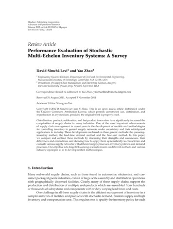
2Advances in Operations ResearchTable 1: Classification of the literature.1234Single-period models or models with zero lead timesSupply chains with capacity limitsOptimal policy characterizationGuaranteed service time modelsModels with positive lead timesUncapacitated supply chainsPolicy evaluation and optimizationStochastic service time modelsproduct at each facility so as to minimize the system-wide inventory cost subject to customerservice requirements. For many years, both practitioners and academicians have recognizedthe potential benefit of effective inventory control in such networks. In fact, the literature onmulti-echelon inventory control can be dated back to the 1950s. However, it is only in the lastfew years that some of these benefits have been realized, see, for example, Lee and Billington 1 , Graves and Willems 2 , and Lin et al. 3 . Three reasons have contributed to this trend: 1 the availability of data, not only on network structure and bill of materials BOMs ,but also on demand processes, transportation lead times and manufacturing cycletimes, and so forth; 2 industry that is searching for scientific methods for inventory management thathelp to cope with long lead times and the increase in customer service expectations; 3 recent developments in modeling and algorithms for the control of general structure multi-echelon inventory systems.These developments are built on three generic methods: the queueing-inventory method, the lead-time demand method, and the flow-unit method. While the first two methodstake a snapshot of the system and focus on quantities e.g., backorders and on-hand inventory , the third method follows the movement of each flow unit and focuses on times e.g.,stockout delays and inventory holding times . This paper discusses the strengths and weaknesses of these methods, differences and connections among these methods, and demonstrates their abilities in handling various network topologies, inventory policies, and demand processes.1.1. Classification of LiteratureTo position our survey in perspective, we classify the related literature by several dimensions see Table 1 .Models with Zero Lead Times versus Models with Positive Lead TimesModels with zero lead times can be used to analyze strategic issues as well as tactical oroperational issues when the lead times can be ignored, see, for example, the celebratedNewsvendor model 4 and some mathematical-programming-based models 5 . Modelswith positive lead times, such as the multi-echelon inventory models, explicitly consider leadtimes and even uncertain lead times.Capacitated Supply Chains versus Uncapacitated Supply ChainsSupply chain models with limited production capacity received significant attention in theliterature. We refer to Kapuscinski and Tayur 6 for a review of multistage single-productsupply chains, to Sox et al. 7 for single stage multiproduct systems, and to Shapiro 5 for
Advances in Operations Research3mathematical programming models of production-inventory systems. In uncapacitated supply chains, we typically assume a positive exogenous “transit time” for processing a job,where the “transit time” is defined as the total time it takes from job inception to job completion. This transit time may represent manufacturing cycle time, transportation lead time,or warehouse receiving and processing times. The literature on uncapacitated supply chainscan be further classified into two categories: i.i.d. or sequential transit time. In the former, thetransit times are i.i.d. random variables; while, in the latter, the transit times are sequential inthe sense that jobs are completed in the same sequence as they are released.Optimal Policy Characterization versus Policy Evaluation and OptimizationThe focus of the former is on identification and characterization of the structure of the optimalinventory policy. We refer to Federgruen 8 , Zipkin 9 , and Porteus 10 for excellentreviews. Unfortunately, the optimal policy is not known for general supply chains except forsome special cases. When the optimal policy is unknown or known but too complex to implement, an alternative approach is to evaluate and optimize simple heuristic policies whichare optimal in special cases but not in general.Guaranteed Service Time Model versus Stochastic Service Time ModelIn the former, it is assumed that in case of stockout, each stage has resources other than theon-hand inventory such as slack capacity and expediting to satisfy demand so that thecommitted service times can always be guaranteed. In the latter, it is assumed that in case ofstockout, each stage fully backorders the unsatisfied demand and fills the demand until onhand inventory becomes available. Thus, the delay due to stockout i.e., the stockout delay israndom, and the committed service times cannot be 100% guaranteed. A recent comparisonbetween the two models is provided by Graves and Willems 11 .1.2. The Scope and Objective of the SurveyThis survey focuses on the stochastic service time model for uncapacitated supply chains.Because we are interested in general supply networks, we focus on policy evaluation andoptimization. Given a certain class of simple but effective inventory policies, the specificproblem that we address in this survey is how to characterize and evaluate system performance in general structure supply chains. The challenge arises from the fact that the inventory policy controlling one product at one facility may have an impact on all other products/facilities in the network either directly or indirectly.For guaranteed service time models, Graves and Willems 11 summarize recentdevelopment and demonstrate its potential applications in industry-size problems. Thesedevelopments are based on the lead-time demand method. For the stochastic service timemodel, Hadley and Whitin 12 provide the first comprehensive review for single-stagesystems. Chen 13 reviews the lead-time demand method in serial supply chains, and de Kokand Fransoo 14 discuss some of its applications in more general supply chains. Song andZipkin 15 provide an in-depth review of the literature on assembly systems, while Axsater 16 presents an excellent survey for serial and distribution systems. Zipkin 9 presentsan excellent and comprehensive review for the queueing-inventory method in single-stagesystems and the lead-time demand method in single-stage, serial, pure distribution, and pureassembly systems.
4Advances in Operations ResearchThe objective of this paper is to compare the effectiveness of queueing-inventorymethod, the lead-time demand method, and the flow-unit method in supply chains along thefollowing dimensions: network topology, inventory policy, and demand process. Specifically,we discuss how to apply each method systematically to evaluate various network topologieswith either i.i.d. or sequential transit times, either base stock or batch ordering inventorypolicy, and either unit or batch demand process. The network topology considered includessingle-stage see Section 2 , serial Section 3.1 , pure distribution Section 3.2 , pure assemblyand 2-level general networks Section 3.3 , and tree and more general networks Section 3.4 .For each network topology, we discuss the three methods side by side and address questionssuch as, how are different stages connected and dependent? How does each method work?How are the results/methods connected to those of single-stage systems and systems ofother topologies? What are the weakness and strength of each method? And what are thedifferences and connections among the methods? Some open questions are summarized inSection 4.While some of the materials covered here appeared in previous reviews, we presentthese materials together with recent results in a coherent way by building connectionsamong different methods and establishing uniform treatment of each method across differentnetwork topologies. We also shed some lights on the strengths and limitations of each method.2. Single-Stage SystemsIn this section, we consider single-stage systems and review the key assumptions and resultsof the three generic methods. We show how each method can handle different inventorypolicies, transit times, and demand processes. Following convention, we define a stage anode, equivalently to be a unique combination of a facility and a product, where the facilityrefers to a processor plus a storage where the latter carries inventory processed by the former.Inventory PoliciesIn this paper, we focus on either continuous-review or periodic-review base-stock and batchordering policies. For any stage in a supply chain, we define inventory position to be the sumof its on-hand inventory and outstanding orders subtracting backorders. Under continuousreview, a base-stock policy with base-stock level s works as follows: whenever inventoryposition drops below s, order up to s. A batch-ordering policy with reorder point r and batchsize Q works as follows: whenever the inventory position drops to or below the reorder pointr, an order of size nQ is placed to raise the inventory position up to the smallest integer abover. Clearly, a base-stock policy is a special case of the batch-ordering policy with a batch sizeQ 1. Continuous-review base-stock policies are often used for expensive products facinglow-volume but highly uncertain demand e.g., service parts . Batch-ordering policies areoften used where economies of scale in production and transportation cannot be ignored commodities .Under periodic review, the base-stock and batch ordering policies work in similarways as their continuous-review counterparts except that inventory is reviewed only oncein one period. The sequence of events is as follows 12 . At the beginning of a review period,the replenishment is received, the inventory is reviewed, and then an order decision is made.Demand arrives during the period. At the end of the period, costs are calculated. Some workin the literature assumes that all demands arrive at the end of the period; see, for example,
Advances in Operations Research5Zipkin 9, Chapter 9 . Under this assumption, a single-stage periodic-review inventorysystem can be viewed as a special case of its continuous-review counterpart with constant demand interarrival times and batch demand sizes. In this survey, we assume demandarrives during the period unless otherwise mentioned.Transit TimesIf the transit times Section 1.1 are sequential and stochastic, namely, “stochastic sequentialtransit times,” then they must be dependent over consecutive orders. Kaplan 17 presents adiscrete-time model for the stochastic sequential transit time in a periodic-review single-stagesystem, where the evolution of the outstanding order vector is modeled by a Markov chain.See Song and Zipkin 18 for a generalization of the model. For continuous-review singlestage systems, Zipkin 19 presents a continuous-time model for stochastic and sequentialtransit times.Definition 2.1. The exogenous, stochastic, and sequential transit times are defined as follows:there exits an exogenous continuous-time stochastic process {U t } that is stationary andergodic with finite limiting moments, such that the sample path of {U t } is left-continuous,the transit time at t, L t U t , and t L t is nondecreasing.Svoronos and Zipkin 20 apply this model to multistage supply chain with twoadditional assumptions: 1 the transit times are independent of the system state, for example,demand and order placement and 2 the transit times are independent across stages.In practice, the transit times can be either parallel or sequential or somewhere inbetween. Many production and transportation processes in the real world are subject torandom exogenous events. Indeed, the orders placed by the systems under considerationmay be a negligible portion of their total workload. Thus, the transit times are exogenous andshould be estimated from data. While in some practical cases, the sequential transit timemodel may be more realistic than the i.i.d. transit time model 20 , in cases such as repairingand maintenance, the i.i.d. transit time model may be a better approximation 21 .Demand ProcessesBoth unit demand and batch demand processes are studied in the literature. On arrival of abatch demand, one shall address questions such as: should all units of the demand be satisfied together unsplit demand ? Or should each demand unit be satisfied separately splitdemand ? For a supply system either production or transportation processing a job ofmultiple units, one needs to address questions like: is the job processed and replenished asan individable entity unsplit supply ? Or is each unit processed and replenished separately split supply ? If the former is true, does the transit time depend on job size? See Zipkin 9 for more discussions on these questions. While the case of split demand is easier to handleand thus widely studied in the literature, the case of unsplit demand is much more difficult;see Section 2.1 for more details.The Basic AssumptionFor the ease of exposition, we make the following assumption throughout the survey unlessotherwise mentioned.
6Advances in Operations ResearchAssumption 2.2. The system is under continuous review; unsatisfied demands are fully backordered; outside suppliers have ample stock; the transit times are exogenous either i.i.d. orsequential; demand is satisfied on a first-come first-serve FCFS basis; demand can be split;supply cannot be split; transit times do not depend on job sizes.Throughout the survey, we use the following notations: a max{a, 0}, a max{ a, 0}. E · , V · are the mean and variance of a random variable, respectively. If randomvariables X and Y are independent, we denote X Y . We consider base-stock policies withs 0 and batch-ordering policies with r 0 unless otherwise mentioned.We define the basic model for single-stage systems as follows: inventory is controlledby a base-stock policy, demand follows Poisson process with rate λ, and the transit time i.e.,lead time L is constant. In the following subsections, we first discuss the methods in the basicmodel and then extend the results to more general demand process, inventory policies, andsupply process.2.1. The Queueing-Inventory MethodLet {IO t , t 0} be the outstanding order process, {IP t , t 0} the inventory positionprocess, and {IL t , t 0} the process of net inventory on-hand minus backorder . Define{I t , t 0} {B t , t 0} to be the process of on-hand inventory backorder, resp. . Forappropriate initial conditions, the following equations hold under Assumption 2.2,IO t IL t IP t ,t 0, 2.1 I t IL t , 2.2 B t IL t . 2.3 For unsplit demand, 2.2 - 2.3 do not hold since I t 0 and B t 0 can hold simultaneously.Note that IO t is the number of jobs in the supply process. The queueing-inventory method characterizes the probability distribution of IO t by identifying the appropriatequeueing analogue. One can follow a 3-step procedure to characterize the system performance: 1 the distribution of IP t , 2 the distribution of IO t , and 3 the dependence ofIO t and IP t . We focus on steady-state analysis and define IO limt IO t . The samenotational rule applies to IL, IP , and I and B.Clearly, IP s for base-stock policies. For batch-ordering policies, the distribution ofIP only depends on the demand process. IP is uniformly distributed in {r 1, r 2, . . . , r Q}for renewal batch demand under mild regularity assumptions 22 . See Zipkin 19 for adiscussion of more general demand processes. The distribution of IO depends on the demandprocess, the inventory policy, and the supply system see discussions below . For batchordering policies, IP depends on IO. Intuitively, the lower the IP , the longer the time sincethe last order, and therefore the lower the IO.i.i.d. Transit TimeConsider first the basic model with constant L, the queueing analogue is a M/D/ queue. ByPalm theorem 23 , IO follows Poisson λL distribution. If L is stochastic, then the queueing
Advances in Operations Research7analogue is a M/G/ queue and IO follows Poisson λE L distribution. Because demandis satisfied on a FCFS basis, the stockout delay differs from L even at s 0; see Muckstadt 24,page 96 for an exact analysis. For renewal unit demand, the queueing analogue is a G/G/ queue. For compound Poisson demand, then the queueing analogue is a MY /G/ queuewhere {Yn } is the demand size process. The distribution of IO is compound Poisson underAssumption 2.2.Consider the basic model but with a batch ordering policy, the queueing analogue isa Er Q /D/ queue where Er stands for Erlang interarrival times. See Galliher et al. 25 foran exact analysis. For batch demand processes, tractable approximations become appealing.One can first assume IP IO and then approximate the distribution of IO by results fromsystems with base-stock policy and batch-demand processes 9, Section 7.2.4 .Sequential Transit TimeConsider the basic model with sequential transit times Definition 2.1 . Let D t1 , t2 be thedemand during time interval t1 , t2 , where t1 t2 , and let D L limt D t L, t . BySvoronos and Zipkin 20 :Proposition 2.3. IO has the same distribution as D L .Proof. See the appendix for a proof.D t L, t D L is called the lead-time demand. If demand follows compoundPoisson process, Proposition 2.3 also holds under Assumption 2.2.For the basic model with constant transit time, one can obtain Proposition 2.3 by analternative approach 9 . At time t, because all orders placed on or before t L are replenishedwhile all orders placed after t L are still in transit, IO t equals to the number of orders placedduring t L, t . Due to the Poisson demand and the continuous-review base-stock policy, onemust haveIO t D t L, t . 2.4 Consider the batch ordering policy in the basic model with sequential transit times Definition 2.1 . Equation 2.4 does not hold because IO t is clearly not the demand during t L, t . In addition, IO t depends on IP t . Exact analysis of these systems using thequeueing-inventory method is rare. Fortunately, such systems can be easily handled by thelead-time demand method and the flow-unit method.2.2. The Lead-Time Demand MethodConsider the basic model. Observe that at time t, the system receives all orders placed on orbefore t L but none of the orders placed after t L, thenIL t IP t L D t L, t . 2.5 Equations 2.2 - 2.3 remain true here. Although 2.5 looks quite similar to 2.1 and 2.4 , they follow completely different logic. Indeed, IL and IP are measured at different
8Advances in Operations Researchtimes t or t L in the lead-time demand method rather than the same time t in the queueing-inventory method.Let {IP tn } be the embedded discrete time Markov chain DTMC formed by observing IP t right after each ordering decision at tn . Zipkin 19 shows the following.Proposition 2.4. Consider a single-stage system. If i the inventory policy depends only on inventory position, ii the demand sizes are i.i.d. random variables independent of the arrival epochs, iii {IP tn , n 0} is irreducible, aperiodic, and positive recurrent, iv the arrival epochs forma counting process which is either stationary or converges to a stationary process in distribution ast , and v the transit times are sequential and exogenous (Definition 2.1), then 1 IP has the same distribution as {IP tn } as n , 2 IL IP D L , 3 IP D L .The inventory policy includes the batch-ordering policy and the s, S policy, andthe demand process includes renewal batch process and the superposition of independentrenewal batch processes 19 . We point out that for 2.5 and Proposition 2.4 to hold, theassumptions of sequential transit time, FCFS rule, and split demand are necessary.In the basic model, the stockout delay, X, for a demand at t, satisfies 26 Pr{X x} Pr{D t Lx, t s},for 0 x L. 2.6 To see this, note that, at t x, all orders triggered by demand on or prior to t x L arereplenished. Because the demand at t has priority over demand after t, the demand at t issatisfied on or before t x if and only if the orders triggered by demand during t x L, t are less than s. By the same logic, for compound Poisson demand, the stockout delay for thekth unit of a demand, X k , is given byPr{X k x} Pr{D t Lx, t s k},for 0 x L. 2.7 Consider now the basic model under periodic review. Let IP n be the inventoryposition at the beginning of period n after order decision is made and IL n I n and B n the net inventory inventory on-hand and backorder at the end of period n after demand isrealized. Let L here be an integer multiple of a review period and D n, m the demand fromperiod n to m inclusive. According to the sequence of events see beginning of Section 2 , 2.5 and 2.2 - 2.3 become IL n IP n L D n L, n , I n IL n , and B n IL n ,respectively. By Hausman et al. 27 , for x L, Pr all demand in period n is satisfied within x periods Pr{D n Lx, n s}. 2.8 2.3. The Flow-Unit MethodFor the basic model, suppose a demand arrives at time t, then the order triggered by thisdemand will satisfy the sth demand after t 28, 29 . Alternatively, the corresponding order
Advances in Operations Research9that satisfies the demand at time t is placed at t T s , where T s is determined by startingat time t, counting backwards until the number of demand arrivals reaches s 30 . We callthe former the “forward method” because, for each order, it looks forward to identify thecorresponding demand. We call the latter the “backward method” because, for each demand,it looks backward to identify the corresponding order.Both methods yield the same result for single-stage systems. For general networks, thetwo methods may take different angles, and thus one can be more convenient than the other Section 3 . We focus on the backward method unless otherwise mentioned. The stockoutdelay, X, for the demand at time t and the holding time, W, for the product that satisfies thisdemand are given byX L T s , 2.9 W T s L . 2.10 Unlike the queueing-inventory method and the lead-time demand method, the flowunit method focuses on the stockout delay the inventory holding time associated witheach demand product rather than the on-hand inventory and backorders at a certain time.Equations 2.9 - 2.10 hold also for stochastic sequential lead times Definition 2.1 and forany point unit-demand process 31 . We should point out that the assumptions of sequentiallead time and FCFS rule are necessary for 2.9 - 2.10 . By 2.9 , the distribution of the stockoutdelay, X, is given by,Pr{X x} Pr{L T s x},for 0 x L. 2.11 For compound Poisson demand, different units in one demand face statistically differentstockout delays 29 . Consider the kth unit of a demand at t, the backorder delay, X k , andthe inventory holding time, W k , for the corresponding item that satisfies this unit areX k L T J k , 2.12 W k T J k L , 2.13 where J k is obtained by starting at time t, counting backwards demand arrivals until thecumulative demand becomes greater than s k in the first time. See Forsberg 32 and Zhao 33 for extended discussions.A comparison between 2.6 - 2.7 and 2.11 - 2.12 demonstrates the connectionsbetween the lead-time demand method and the flow-unit method. Because D t L, t is thecumulative demand and T s is the sum of interarrival times, the event {T s L x} isequivalent to the event {D t L x, t s} for unit demand 34, page 406 . Similarly, theevent {T J k L x} is equivalent to the event {D t L x, t s k} for batch demand.For the basic model under periodic review, if demand arrives at the end of each period,then the system is a special case of its continuous-review counterpart 33 . If demand arrives
10Advances in Operations Researchduring a period, the flow-unit method also applies, see, for example, Axsater 35 . For thebasic model with batch ordering policy, by Axsater 36 ,X L T S ,W T S L , 2.14 where S is a random integer uniformly distributed in {r 1, r 2, . . . , r Q}. See also Zhaoand Simchi-Levi 30 . For the basic model with both batch ordering policy and compoundPoisson demand, the analysis is more involved but still tractable, see Axsater 37 .3. Multistage Supply ChainsMultistage supply chains differ from single-stage systems because the lead time at one stagedepends on other stages’ stock levels. For a stage, the lead time is the total time neededfrom order placement to order delivery. Clearly, lead times include but are not limited tothe “transit times.”Notation 1. Consider a supply chain under Assumption 2.2 with node set N and arc set A. Anarc refers to a pair of nodes with direct supply-demand relationship. We define the following. i {IOj t , t 0}: the outstanding order process at node j N. ii {IPj t , t 0}: the inventory position process at node j. iii {ILj t , t 0}: the net inventory on-hand minus backorder process at node j. iv {Ij t , t 0} {Bj t , t 0} : the process of on-hand inventory backorder at nodej. v Lj Li,j : the processing cycle time at node j transportation lead time over arc i, j A . vi ITj ITi,j : the inventory in-transit during Lj during Li,j . j : the total replenishment lead time at node j. vii L viii Xj Wj : the stockout delay inventory holding time at node j. ix τj αj , βj : the committed service time target type 1, 2 service at node j. x ai,j : the BOM structure, that is, one unit at node j requires ai,j unit s from node i. xi hj πj : the inventory holding cost penalty cost per unit item per unit time at nodej. xii sj rj , Qj : base-stock level reorder point, batch size at node j.3.1. Serial SystemsIn this section, we extend the methodologies and results of the single-stage systems to a serialsupply chain where nodes j J are numbered by 1, 2, . . . , J . Node J receives externalsupply, node j 1 supplies node j, and node 1 supplies external demand. The transit timeof node J is L J , and the transit time between stage j 1 and j is Lj . This system can becontrolled either by an installation policy or an echelon policy. For an installation policy, thenotation is defined as above. For an echelon policy, we need the following notation.
Advances in Operations Research11 i IPje : the echelon inventory position at stage j, which is the sum of inventory onhand and on-order at stage j plus inventory on-hand and in-transit at all downstream stages of j subtracting B1 . ii ILej IPje IOj : the echelon net inventory at stage j. iii Ije ILej iv ITje ITjB1 : the echelon on-hand inventory.ILej : the echelon inventory in-transit. v sej rje : the echelon base-stock level reorder point .An echelon batch-ordering policy works as follows: whenever IPje drops to or below rje , anorder of size nQj is placed to raise the echelon inventory position up to the smallest integerabove rje . According to convention, we assume that Qj 1 and rj 1 are integer multiples of Qjfor all j.We define the basic model for se
product at each facility so as to minimize the system-wide inventory cost subject to customer service requirements. For many years, both practitioners and academicians have recognized the potential benefit of effective inventory control in such networks. In fact, the literature on multi-echelon inventory control can be dated back to the 1950s.