Transcription
Linear FilteringGoal: Provide a short introduction to linear filtering that is directly relevant for computer vision.Here the emphasis is on: the definition of correlation and convolution, using convolution to smooth an image and interpolate the result, using convolution to compute (2D) image derivatives and gradients, computing the magnitude and orientation of image gradients.We discuss how the filters we use in 2D images can be extended to compute spatiotemporal gradientsfor videos.Finally, we introduce the concept of the gradient tensor, along with its magnitude and spatial orientation. We show the application of gradient tensors to colour images.Readings: Szeliski, Section 3.2 [optional: 3.4-5].CSC420: Linear Filteringc Allan Jepson, Sept. 2011Page: 1
Correlation for 1D SignalsSignal I(k)kjFilter f(*) recentered at pixel j,(f( 1), f(0), f(1)) ( 0.5, 0, 0.5)r(j)Response r(k)kjThe correlation of the filter f (k) with the image I(k) is the new signal r(k) defined byr(j) KXf (s)I(j s).s KHere f (k) is assumed to be zero for k larger than the filter radius K.Figure is from James Sewart’s filtering applet: http://research.cs.queensu.ca/ jstewart/applets/filter/filter.htmlCSC420: Linear FilteringPage: 2
Correlation and ConvolutionDefn. The correlation of a 2D filter f with a monochromatic (i.e., grayscale) image I:Correlation: r(j, k) KKXXf (s, t)I(j s, k t).s K t KHere f (j, k) is zero for j or k larger than the filter radius K.Intuitively, to compute the correlation response r(j, k), re-center the filter so that f (0, 0) is “aligned” with I(j, k) (see 1D example on previous page), pointwise multiply the filter and the image values at each pixel (for which f 6 0), sum these products to form r(j, k).Defn. The convolution of a 2D filter f with an image I:Convolution: r(j, k) KKXXs K t Kf ( s, t)I(j s, k t).(1)We denote convolution as r f I. Note f I is the same as correlation using the flipped filter kernel,i.e., g(j, k) f ( j, k). For historical reasons we emphasize convolution over correlation.CSC420: Linear FilteringPage: 3
Image Boundary TreatmentsCentered filter kernel.Image fromElder et al, 1998.When the filter kernel extends beyond the edge of the image, we use a boundary treatment.Options for this include (see upConv in the Matlab iseToolbox): repeat, use the nearest image pixel within the image boundary; reflect the image across its boundaries; zero, use zero for any pixel beyond the image boundary; dont-compute the response when the re-centered filter extends beyond the filter boundary.We often use the repeat rule, but care must be taken interpreting the response near the image boundary.CSC420: Linear FilteringPage: 4
Separable Filter KernelsThe direct implementation of the convolution of a L L filter kernel with an N M image requiresO(L2N M ) operations.The same convolution can also be obtained using the Fast Fourier Transform (typically with a periodicboundary treatment) in O(N M log(N M )) operations.We can often use separable filter kernels which, by definition, can be written as a product of twofunctions of only one variable each, that is,f (j, k) f1(j)f2(k).It can be shown that r f I f1 (f2 I). These two successive 1D convolutions require onlyO(LN M ) operations (compared to O(L2N M ) for the direct approach) and allow for the use of all theprevious boundary treatments.Due to the use of image pyramids (see Szeliski, Sec. 3.5) the size, L, of the filter kernels can typicallybe kept reasonably small.CSC420: Linear FilteringPage: 5
Kernels with Real-Valued ArgumentsConsider a filter kernel f ( x) defined over a continuous range of values, x (x, y)T R2. As before,assume f ( x) 0 outside the range [ K, K] [ K, K].Given such a kernel, it is useful to change variables in the definition of convolution, namely equation(1). In particular, replace (j, k) by real-valued variables (x, y), and set m x s, and n y t (bothinteger-valued). With this change of variables in, we find from (1) thatXr( x) f (x m, y n)I(m, n).(2)m,n Z2 ,f 6 0Here the image I(j, k) is always evaluated at integer-valued points (i.e., pixels or “grid points”), butthe result r( x) can now be evaluated for real-valued points.The idea in (2) is simply to center the flipped kernel at any real-valued x rather than only at integervalued pixel coords.CSC420: Linear FilteringPage: 6
Applications of Kernels with Real-Valued DomainsFiltering and Interpolation. Let the filtered image be r( x) f ( x) I. Since x here is a continuousvariable, we can clearly sample r( x) at a higher rate than the original image. That is, we can interpolatethe filtered image r( x).Note, we are interpolating r( x), not the original image I(j, k). To do the latter we need to ensure thatthe filter kernel is chosen such that r(j, k) I(j, k). (Optional further reading.)Spatial Deriviatives. It also follows that the x and y derivatives of r( x), namely rx( x) and ry ( x),satisfyrx( x) fx I, and ry ( x) fy I,where fx( x) and fy ( x) are the x and y derivatives of the kernel f ( x).CSC420: Linear FilteringPage: 7
Example: Clipped Gaussian FilterClipped Gaussian Kernel, σ 2.0Derivative Kernel, σ 2.00.05gx(x; σ)g(x; σ)0.20.10 8 6 4 2 0 2 4x and k in pixels680 0.05 8 6 4 2 0 2 4x and k in pixels68For example, consider the 1D clipped Gaussian kernel:(22Ce x /(2σ ), for K x K,g(x; σ) 0,otherwise.(3)Here x R and σ 1 is the scale parameter, it is proportional to the width of the kernel in x, K 0 is an integer specifying the radius in which the kernel is non-zero, typically K 3σ,P x2 /(2σ 2 )e, which normalizes g(x; σ) to sum to one over all integer arguments. 1/C Kk KThe kernel g(x; σ) and its first derivative gx(x; σ) (ignoring the discontinuities) are shown above.CSC420: Linear FilteringPage: 8
Image SmoothingConvolution with the 2D clipped Gaussian filter kernel, g( x; σ) g(x; σ)g(y; σ), blurs the image:Using:σ 2The kernel g( x; σ) is shown in the bottom right corner of the smoothed image, and is circularly symmetric (modulo the clipping at K).CSC420: Linear FilteringPage: 9
Image DerivativesThe blurred image along with its x and y derivatives are shown below. The dominant grey tone in thederivative images denotes a response of zero, with positive (negative) values being lighter (darker).xyThe x and y derivative filters are gx( x) gx(x)g(y) and gy ( x) g(x)gy (y) (see the inlaid images inthe bottom-right corners).CSC420: Linear FilteringPage: 10
Image GradientThe gradient of an image r( x) is defined to be the following 2-vector at every point x,! x) rx( x) . r( ry ( x)Disc Imagex-derivativey-derivativeGradient Magnitude(4)Gradient OrientationxyThe magnitude of the gradient S( x) is defined to be the vector 2-norm of the gradient, namely S( x) x) (rx( x)2 ry ( x)2)1/2. The magnitude is zero only if both the x and y derivatives of r( x) r( vanish. x) is nonzero, the gradient (vector) at x is in the “steepest ascent” direction (i.e., theWhen r( direction r( x) increases the fastest). We define the gradient angle as θ atan2(ry ( x), rx( x)), and the x)/ r( x) .gradient direction to be u(θ) (cos(θ), sin(θ))T r( CSC420: Linear FilteringPage: 11
Image GradientThe gradient identifies the local magnitude and direction of variation in the blurred image r( x).Original ImageGradient MagnitudeGradient OrientationColour KeyThe only remaining parameter here is the scale parameter σ (we used σ 2). As σ increases theoriginal image is increasingly blurred, and detail is lost. On the other hand, the responses are lesssensitive to image noise, and will have better performance on smooth ramps in the image.CSC420: Linear FilteringPage: 12
Image Gradient: Fine ScaleThe results for σ 1 are shown below.Original ImageGradient MagnitudeGradient OrientationColour KeyCompare these results with those for σ 2 (previous slide). While the detail is significantly sharperhere (for σ 1), the gradient directions are more sensitive to image noise (e.g., on the jagged edgesand within the soft shadows in the original image). See Elder et al, 1998, for automatic scale selection.CSC420: Linear FilteringPage: 13
Spatiotemporal ImagesA sequence of video images forms a space-time volume image.txOne video frame of pedestriansyFrom Niyogi and Adelson, 1994.Gradients, gradient magnitude and orientation, can all be measured as before, for example, using aseparable filter g( x, t) g(x; σ)g(y; σ)g(t; σ) along with its x, y, and t derivatives. Gradients againpoint in the “steepest ascent” direction, perpendicular to 2D surfaces of constant brightness in ( x, t).CSC420: Linear FilteringPage: 14
Multispectral Images x) (I1( x), . . . , In( x))T . For example, an RGB image has n 3.Consider an n-dimensional image I( We could form a n 4 dimensional image by adding an infrared channel, say.Hats ImageRGB SpaceRed (R) ComponentGreen (G) ComponentRGB SpaceBlue (B) ComponentRGB Space (View Along Gray Axis)RGB-space is a cube, with each side of length 255 (for 8-bit images). The gray axis is the diagonalfrom (0, 0, 0)T (Black) to (255, 255, 255)T (White).CSC420: Linear FilteringPage: 15
Projecting Multispectral Images to Monochromatic x) (I1( x), . . . , In( x))T our previous filtering techniques can be appliedFor an n-dimensional image I( x)), where h is a (smooth) mapping from Rn to R.to any monochromatic image h(I( For example, a simple form for h is a linear mapping, w h(I) T I,where w is a constant n-vector (aka the projection direction).Suitable projection directions w can be selected to highlight different aspects of the original image I x).in the monochromatic image w T I( We illustrate the monochrome images obtained from several different projection directions in the nexttwo slides.CSC420: Linear FilteringPage: 16
Colour-Opponent ChannelsFor example, consider choosing projection directions to (roughly) decorrelate a typical RGB imageI (IR , IG, IB )T . Define IBrIR Brightness1/ 3 1/ 3 1/ 3 IY B C IG , where C 1/ 6 1/ 6 2/ 6 . R G - 2B, aka Y-B (5) 01/ 2 1/ 2IRGIB R-GThis matrix C is a unitary transformation of the RGB coordinates, i.e., C T C I (note det(C) 1).This transformation very roughly decorrelates the RGB channels (see colourTutorial.m in theutvis toolbox). x) where wNote each component of the transformed image vector, say IY B , has the form w T I( T is thecorresponding row of C.Caution: A significant amount of research has been done on colour spaces. The mapping C aboveis greatly simplified and is not meant to be an optimal choice. (For more information about colourspaces, begin by looking up “Color model” in Wikipedia.)CSC420: Linear FilteringPage: 17
Example: Colour Opponent ChannelsThese colour opponent channels are illustrated in the following example.Hats ImageRed (R) ComponentGreen (G) ComponentBlue (B) ComponentBrightness ComponentY-B ComponentR-G ComponentNote the R and G images appear very similar, indicating a typically strong correlation. Also note that,in each of the monochromatic images, there are small image regions where the boundaries of the hatshave low contrast. For these regions the gradients will be either small or dominated by other structurein the region. Thus it may be hard to find a single projection direction, w R3, for which the hat x)/ w .boundaries all have large gradients in the single monochromatic image w T I( CSC420: Linear FilteringPage: 18
Image Gradient Tensors: Magnitude and (Spatial) Direction x) simultaneously.Alternatively, it is possible to consider all n channels of I( I x .This is an n 2 matrix (aka tensor), with the k th row given by the x k ( x)]T (Ik,x( x), Ik,y ( x)).and y derivatives of Ik , that is, (Jk,1( x), Jk,2( x)) [ IConsider the Jacobian J( x) The gradient tensor magnitude, S( x), and direction, u(θ( x)), are defined usingS( x) max RJ( x) u(φ) , θ( x) arg max RJ( x) u(φ) ,0 φ π0 φ π(6)where u(φ) (cos(φ), sin(φ))T , · denotes the usual 2-norm, and R is a selected n n weightingmatrix. The gradient direction is then u(θ( x)) (aka, the right principal vector of the weighted Jacobian,RJ( x)). See DiZenzo, 1986, for a closed form solution of θ( x).Note that, in contrast to the gradient direction in monochromatic images, the gradient tensor directionis only defined up to a sign. That is, both u(θ( x)) and u(θ( x)) are solutions.CSC420: Linear FilteringPage: 19
Image Gradient Tensors: Left Principal VectorThe left principal vector of the weighted Jacobian RJ( x) is defined to bew( x) 1RJ( x) u(θ( x)).S( x)(7)This w( x) Rn is, in a sense, a locally optimal choice for the projection vector w discussed above. x)/ w ,To see this optimality, consider the monochromatic image Hw ( x) w T RI( where w is aconstant vector. Here we have divided by w to avoid a trivial dependence of the gradient magnitudeof Hw ( x) on the magnitude of w Then it follows that, at every x, the left principal vector maximizes the (monochromatic) gradientmagnitude over all images of the form Hw ( x). We omit the proof of this (but hint that the interestedreader should consider the singular value decomposition (SVD) of the gradient tensor RJ( x)).For scalar images (i.e., n 1 and R 1), this definition of the gradient tensor magnitude and direction agrees with our previous definition, with the one exception that the gradient tensor direction isindependent of sign. In particular, it can point in the steepest ascent or descent direction.CSC420: Linear FilteringPage: 20
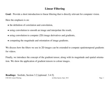
Example Using Gradient TensorsBrightness ImageGradient MagnitudeGradient OrientationOriginal ImageGradient Tensor MagnitudeGradient Tensor OrientationHere we used R diag([1, 4, 4])C (borrowing diag(·) from Matlab) to emphasize the colour opponentchannels over the brightness channel. Note that the hat boundaries are all clearly defined in the gradienttensor approach, which is not true of the results from the brightness image alone. This illustrates theadaptive selection of the left principal direction w( x) that is inherent in this approach.CSC420: Linear FilteringPage: 21
Further InformationLinear filtering is a rich subject, of which we have (intentionally) given only a brief sketch. Importantsubjects that students can entirely skip in this course include: Fourier analysis, sampling, and aliasing, signal interpolation (more generally), upsampling and downsampling signals, filter design,The textbook by Castleman, 1995, provides an excellent introductory treatment of most of these topics(for any student interested in further study outside of this course).Alternatively, Sections 3.2 and 3.4-6 of the textbook by Szeliski provide more information, whileSection 3.8 provides an excellent set of pointers into recent literature.CSC420: Linear FilteringPage: 22
ReferencesCastleman, K.R., Digital Image Processing, Prentice Hall, 1995Silvano Di Zenzo, A Note on the Gradient of a Multi-Image, ComputerVision, Graphics, and Image Processing, 33, 1986, pp.116-125.James Elder and Steven Zucker, Local Scale Control for Edge Detection and Blur Estimation, IEEE Transactions on PAMI, 20(7), 1998,pp.699-716.Sourabh Niyogi and Edward Adelson, Analyzing Gait With Spatiotemporal Surfaces, In IEEE Workshop on Motion of Non-Rigid and Articulated Objects, 1994, pp.64-69.CSC420: Linear FilteringNotes: 23
Linear Filtering Goal: Provide a short introduction to linear filtering that is directly re levant for computer vision. Here the emphasis is on: the definition of correlation and convolution, using convolution to smooth an image and interpolate the result, using convolution to compute (2D) image derivatives and gradients,