Transcription
Deconvolving Feedback Loopsin Recommender SystemsAyan SinhaPurdue Universitysinhayan@mit.eduDavid F. GleichPurdue Universitydgleich@purdue.eduKarthik RamaniPurdue Universityramani@purdue.eduAbstractCollaborative filtering is a popular technique to infer users’ preferences on newcontent based on the collective information of all users preferences. Recommendersystems then use this information to make personalized suggestions to users. Whenusers accept these recommendations it creates a feedback loop in the recommendersystem, and these loops iteratively influence the collaborative filtering algorithm’spredictions over time. We investigate whether it is possible to identify itemsaffected by these feedback loops. We state sufficient assumptions to deconvolvethe feedback loops while keeping the inverse solution tractable. We furthermoredevelop a metric to unravel the recommender system’s influence on the entireuser-item rating matrix. We use this metric on synthetic and real-world datasetsto (1) identify the extent to which the recommender system affects the final ratingmatrix, (2) rank frequently recommended items, and (3) distinguish whether auser’s rated item was recommended or an intrinsic preference. Our results indicatethat it is possible to recover the ratings matrix of intrinsic user preferences using asingle snapshot of the ratings matrix without any temporal information.1IntroductionRecommender systems have been helpful to users for making decisions in diverse domains suchas movies, wines, food, news among others [19, 23]. However, it is well known that the interfaceof these systems affect the users’ opinion, and hence, their ratings of items [7, 24].Thus, broadlyspeaking, a user’s rating of an item is either his or her intrinsic preference or the influence of therecommender system (RS) on the user [2]. As these ratings implicitly affect recommendations to otherusers through feedback, it is critical to quantify the role of feedback in content personalization [22].Thus the primary motivating question for this paper is: Given only a user-item rating matrix, is itpossible to infer whether any preference values are influenced by a RS? Secondary questions include:Which preference values are influenced and to what extent by the RS? Furthermore, how do werecover the true preference value of an item to a user?We develop an algorithm to answer these questions using the singular value decomposition (SVD)of the observed ratings matrix (Section 2). The genesis of this algorithm follows by viewing theobserved ratings at any point of time as union of true ratings and recommendations:Robs Rtrue Rrecom(1)where Robs is the observed rating matrix at a given instant of time, Rtrue is the rating matrix dueto users’ true preferences of items (along with any external influences such as ads, friends, and soon) and Rrecom is the rating matrix which indicates the RS’s contribution to the observed ratings.Our more formal goal is to recover Rtrue from Robs . But this is impossible without strong modelingassumptions; any rating is just as likely to be a true rating as due to the system.Thus, we make strong, but plausible assumptions about a RS. In essence, these assumptions prescribea precise model of the recommender and prevent its effects from completely dominating the future.30th Conference on Neural Information Processing Systems (NIPS 2016), Barcelona, Spain.
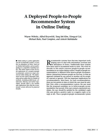
With these assumptions, we are able to mathematically relate Rtrue and Robs . This enables us tofind the centered rating matrix Rtrue (up to scaling). We caution readers that these assumptionsare designed to create a model that we can tractably analyze, and they should not be consideredlimitations of our ideas. Indeed, the strength of this simplistic model is that we can use its insightsand predictions to analyze far more complex real-world data. One example of this model is thatthe notion of Rtrue is a convenient fiction that represents some idealized, unperturbed version of theratings matrix. Our model and theory suggests that Rtrue ought to have some relationship with theobserved ratings, Robs . By studying these relationships, we will show that we gain useful insightsinto the strength of various feedback and recommendation processes in real-data.In that light, we use our theory to develop a heuristic, but accurate, metric to quantitatively infer theinfluence of a RS (or any set of feedback effects) on a ratings matrix (Section 3). Additionally, wepropose a metric for evaluating the influence of a recommender system on each user-item rating pair.Aggregating these scores over all users helps identify putative highly recommended items. The finalmetrics for a RS provide insight into the quality of recommendations and argue that Netflix had abetter recommender than MovieLens, for example. This score is also sensitive to all cases where wehave ground-truth knowledge about feedback processes akin to recommenders in the data.2Deconvolving feedbackWe first state equations ans assumptions under which the true rating matrix is recoverable (ordeconvolvable) from the observed matrix, and provide an algorithm to deconvolve using the SVD.2.1A model recommender systemConsider a ratings matrix R of dimension m n where m is the number ofusers and n is the number of items beingrated. Users are denoted by subscript u,and items are denoted by subscript i, i.e.,Ru,i denotes user u’s rating for item i. Asstated after equation (1), our objectiveis to decouple Rtrue from Rrecom giventhe matrix Robs . Although this problemseems intractable, we list a series of as- Figure 1: Subfigure A shows a ratings matrix with recsumptions under which a closed form ommender induced ratings and true ratings; Figure B:solution of Rtrue is deconvolvable from Feedback loop in RS wherein the observed ratings is afunction of the true ratings and ratings induced by a RSRobs alone.Assumption 1 The feedback in the RS occurs through the iterative process involving the observedratings and an item-item similarity matrix S: 1Robs Rtrue H (Robs S).(2)Here indicates Hadamard, or entrywise product, given as: (H R)u,i Hu,i · Ru,i . This assumptionis justified because in many collaborative filtering techniques, Rrecom is a function of the observedratings Robs and the item-item similarity matrix, S . The matrix H is an indicator matrix over a setof items where the user followed the recommendation and agreed with it. This matrix is essentiallycompletely unknown and is essentially unknowable without direct human interviews. The model RSequation (2) then iteratively updates Robs based on commonly rated items by users. This key idea isillustrated in Figure 1. The recursion progressively fills all missing entries in matrix Robs startingfrom Rtrue . The recursions do not update Rtrue in our model of a RS. If we were to explicitly considerthe state of matrix Robs after k iterations, Rk 1obs we get: k 1(k)kk 1Robs Rtrue H(Robs Sk ) Rtrue H(k)Rtrue H(k 1) (RobsSk 1 ) Sk . . . (3)Here Sk is the item-item similarity matrix induced by the observed matrix at state k. The aboveequation 3 is naturally initialized as R1obs Rtrue along with the constraint S1 Strue , i.e, the similarity1RTobsFor an user-user similarities, Ŝ, the derivations in this paper can be extended by considering the expression: RTtrue HT (RTobs Ŝ). We restrict to item-item similarity which is more popular in practice.2
matrix at the first iteration is the similarity matrix induced by the matrix of true preferences, Rtrue .Thus, we see that Robs is an implicit function of Rtrue and the set of similarity matrices Sk , Sk 1 , . . . S1 .Assumption 2 Hadamard product H(k) is approximated with a probability parameter αk (0, 1].We model the selection matrix H(k) and it’s Hadamard problem in expectation and replace thesuccessive matrices H(k) with independent Bernoulli random matrices with probability αk . Takingthe expectation allows us to replace the matrix H(k) with the probability parameter αk itself: kk 1Rk 1(4)obs Rtrue αk (Robs Sk ) Rtrue αk Rtrue αk 1 (Robs Sk 1 ) Sk . . .The set of Sk , Sk 1 , · · · are apriori unknown. We are now faced with the task of constructing a validsimilarity metric. Towards this end, we make our next assumption.(obs)Assumption 3 The user mean R̄u in the observed and true matrix are roughly equal: R̄uThe Euclidean item norms kRi k are also roughly equal: kR(obs)k kR(true)k.ii(true) R̄u.These assumptions are justified because ultimately we are interested in relative preferences of itemsfor a user and unbiased relative ratings of items by users. These can be achieved by centeringusers and the normalizing item ratings, respectively, in the true and observed ratings matrices. Wequantitatively investigate this assumption in the supplementary material. Using this assumption, thesimilarity metric then becomes:Pu U (Ru,i R̄u )(Ru, j R̄u )(5)S(i, j) qqPP22u U (Ru,i R̄u )u U (Ru, j R̄u )This metric is known as the adjusted cosine similarity, and preferred over cosine similarity because itmitigates the effect of rating schemes over users [25]. Using the relations R̃u,i Ru,i R̄u , and, R̂u,i R̃u,iR R̄ P u,i u 2 , the expression of our recommender (4) becomes:k R̃ ku U (Ru,i R̄u )iTTTR̂obs R̂true (I f1 (a1 ) R̂true R̂true f2 (a2 )( R̂true R̂true )2 f3 (a3 )( R̂true R̂true )3 . . .)(6)Here, f1 , f2 , f3 . . . are functions of thePprobability parameters ak [α1 , α2 , . . . αk , . . .] of the formfz (az ) cαc11 αc12 . . . αckk . . . such that k ck z, and c is a constant. The proof of equation 6 isin the supplementary material. We see that the centering and normalization results in R̂obs beingexplicitly represented in terms of R̂true and coefficients f (a). It is now possible to recover R̂true , butthe coefficients f (a) are apriori unknown. Thus, our next assumption.Assumption 4 fz (az ) αz , i.e., the coefficients of the series (6) are induced by powers of a constantprobability parameter α (0, 1].Note that in recommender (3), Robs becomes denser with every iteration, and hence the higher orderHadamard products in the series fill fewer missing terms. The effect of absorbing the unknowableprobability parameters, αk ’s into single probability parameter α is similar. Powers of α, producesuccessively less of an impact, just as in the true model. The governing expression now becomes:TTTR̂obs R̂true (I α R̂true R̂true α2 ( R̂true R̂true )2 α3 ( R̂true R̂true )3 . . .)(7)In order to ensure convergence of this equation, we make our final assumption.TAssumption 5 The spectral radius of the similarity matrix α R̂true R̂true is less than 1.TThis assumption enables us to write the infinite series representing R̂obs , R̂true (I α R̂true R̂true TTTα2 ( R̂true R̂true )2 α3 ( R̂true R̂true )3 . . .) as (1 α R̂true R̂true ) 1 . It states that given α, we scale the matrixTTR̂true R̂true such that the spectral radius of α R̂true R̂true is less than 1 2 . Then we are then able to recoverTR̂true up to a scaling constant.Discussion of assumptions. We now briefly discuss the implications of our assumptions. First,assumption 1 states the recommender model. Assumption 2 states that we are modeling expected2See [10] for details on scaling similarity matrices to ensure convergence3
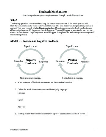
Figure 2: (a) to (f): Our procedure for scoring ratings based on the deconvolved scores with trueinitial ratings in cyan and ratings due to recommender in red. (a) The observed and deconvolvedratings. (b) The RANSAC fit to extract straight line passing through data points for each item. (c)Rotation and translation of data points using fitted line such that the scatter plot is approximatelyparallel to y-axis and recommender effects are distinguishable along x-axis. (d) Scaling of data pointsused for subsequent score assignment. (e) Score assignment using the vertex of the hyperbola withslope θ 1 that passes through the data point. (f) Increasing α deconvolves implicit feedback loopsto a greater extent and better discriminates recommender effects as illustrated by the red points whichshow more pronounced deviation when α 1.behavior rather than actual behavior. Assumptions 3-5 are key to our method working. Theyessentially state that the RS’s effects are limited in scope so that they cannot dominate the world.This has a few interpretations on real-world data. The first would be that we are considering theimpact of the RS over a short time span. The second would be that the recommender effects areessentially second-order and that there is some other true effect which dominates them. We discussthe mechanism of solving equation 7 using the above set of five assumptions next.2.2The algorithm for deconvolving feedback loopsTheorem 1 Assuming the RS follows (7), α is between 0 and 1, and the singular value decompositionof the observed rating matrix is, R̂obs UΣobs V T , the deconvolved matrix Rtrue of true ratings isgiven as UΣtrue V T , where the Σtrue is a diagonal matrix with elements:σtruei 1 2ασobsis124α2 (σobsi ) 1α(8)The proof of the theorem is in the supplementary material. In practical applications, the feedbackloops are deconvolved by taking a truncated-SVD (low rank approximation) instead of the completedecomposition. In this process, we naturally concede accuracy for performance. We consider thematrix of singular values Σ̃obs to only contain the k largest singular values (the other singular valuesare replaced by zero). We now state Algorithm 1 for deconvolving feedback loops. The algorithm issimple to compute as it just involves a singular value decomposition of the observed ratings matrix.3Results and recommender system scoringWe tested our approach for deconvolving feedback loops on synthetic RS, and designed a metric toidentify the ratings most affected by the RS. We then use the same automated technique to studyreal-world ratings data, and find that the metric is able to identify items influenced by a RS.4
Algorithm 1 Deconvolving Feedback LoopsInput: Robs , α, k, where Robs is observed ratings matrix, α is parameter governing feedback loopsand k is number of singular valuesOutput: R̂true , True rating matrix1: Compute R̃obs given Robs , where R̃obs is user centered observed matrix 12: Compute R̂obs R̃obs D 1N , where R̂obs is item-normalized rating matrix, and DN is diagonal matrix of item-normsDN (i, i) qPu U (Ru,iT R̄u )23: Solve UΣobs V S V D( R̂obsr, k), the truncated SVD corresponding to k largest singular values.4: Perform σtrue i5: return U, Σtrue , V 12ασobsi 124α2 (σobsi ) 1 αfor all iTFigure 3: Results for a synthetic RS with controllable effects. (Left to right): (a) ROC curves byvarying data sparsity (b) ROC curves by varying the parameter α (c) ROC curves by varying feedbackexponent (d) Score assessing the overall recommendation effects as we vary the true effect.3.1Synthetic data simulating a real-world recommender systemWe use item response theory to generate a sparse true rating matrix Rtrue using a model related to thatin [12]. Let au be the center of user u’s rating scale, and bu be the rating sensitivity of user u. Let tibe the intrinsic score of item i. We generate a user-item rating matrix as:Ru,i L[au bu ti ηu,i ](9)where L[ω] is the discrete levels function assigning a score in the range 1 to 5: L[ω] max(min(round(ω), 5), 1) and ηu,i is a noise parameter. In our experiment, we draw au N(3, 1),bu N(0.5, 0.5), tu N(0.1, 1), and ηu,i N(0, 1), where N is a standard normal, and is a noiseparameter. We sample these ratings uniformly at random by specifying a desired level of ratingsparsity γ which serves as the input, Rtrue , to our RS. We then run a cosine similarity based RS,progressively increasing the density of the rating matrix. The unknown ratings arePiteratively updatedusing the standard item-item collaborative filtering technique [8] as Rk 1u,i kkj i (si, j Ru, j )kj i ( si, j )P, where kis the iterationnumber and R Rtrue , and the similarity measure at the k iteration is given asP0ski, j Pu URku,i Rku, jqPk 2u U (Ru,i )u U(Rku, j )2th. After the kth iteration, each synthetic user accepts the top r recommen-edations with probability proportional to (Rk 1u,i ) , where e is an exponent controlling the frequencyof acceptance. We fix the number of iterative updates to be 10, r to be 10 and the resulting ratingmatrix is Robs . We deconvolve Robs as per Algorithm 1 to output R̂true . Recall, R̂true is user-centeredand item-normalized. In the absence of any recommender effects Rrecom , the expectation is that R̂trueis perfectly correlated with R̂obs . The absence of a linear correlation hints at factors extraneous tothe user, i.e., the recommender. Thus, we plot R̂true (the deconvolved ratings) against the R̂obs , andsearch for characteristic signals that exemplify recommender effects (see Figure 2a and inset).3.2A metric to assess a recommender systemWe develop an algorithm guided by the intuition that deviation of ratings from a straight line suggestrecommender effects (Algorithm 2). The procedure is visually elucidated in Figure 2. We considerfitting a line to the observed and deconvolved (equivalently estimated true) ratings; however, ourexperiments indicate that least square fit of a straight line in the presence of severe recommendereffects is not robust. The outliers in our formulation correspond to recommended items. Hence, weuse random sample consensus or the RANSAC method [11] to fit a straight line on a per item basis5
Table 1: Datasets and parametersDatasetUsersItemsMin RPIRatingk in eerAdvocateRateBeerFine FoodsWine 1500150015000.22230.15260.12090.16010.2661(Figure 2b). All these straight lines are translated and rotated so as to coincide with the y-axis asdisplayed in Figure 2c. Observe that the data points corresponding to recommended ratings pop outas a bump along the x-axis. Thus, the effect of the RANSAC and rotation is to place the ratings intoa precise location. Next, the ratings are scaled so as to make the maximum absolute values of therotated and translated R̆true , R̆obs , values to be equal (Figure 2d).The scores we design are to measure “extent” into the x-axis. But we want to consider some allowablevertical displacement. The final score we assign is given by fitting a hyperbola through each ratingviewed as a point: R̆true , R̆obs . A straight line of slope, θ 1 passing through the origin is fixed as anasymptote to all hyperbolas. The vertex of this hyperbola serves as the score of the correspondingdata point. The higher the value of the vertex of the associated hyperbola to a data point, the morelikely is the data point to be recommended item. Using the relationship between slope of asymptote,and vertex of hyperbola, the score s( R̆true , R̆obs ) is given by:q22(10)s( R̆true , R̆obs ) real( R̆true R̆obs )We set the slope of the asymptote, θ 1, because the maximum magnitudes of R̆true , R̆obs are equal(see Figure 2 d,e). The overall algorithm is stated in the supplementary material. Scores are zero ifthe point is inside the hyperbola with vertex 0.3.3Identifying high recommender effects in the synthetic systemWe display the ROC curve of our algorithm to identify recommended products in our syntheticsimulation by varying the sparsity, γ in Rtrue (Figure 3a), varying α (Figure 3b), and varying exponente (Figure 3c) for acceptance probability. The dimensions of the rating matrix is fixed at [1000, 100]with 1000 users and 100 items. Decreasing α as well as γ has adversarial effects on the ROC curve,and hence, AUC values, as is natural. The fact that high values of α produce more discriminativedeconvolved ratings is clearly illustrated in Figure 2 f. Additionally, Figure 3 d shows that thecalculated score varies linearly with the true score as we change the recommender exponent, e, colorcoded in the legend. Overall, our algorithm is remarkably successful in extracting recommendeditems from Robs without any additional information. Also, we can score the overall impact of the RS(see the upcoming section RS scores) and it accurately tracks the true effect of the RS.3.4Real dataIn this subsection we validate our approach for deconvolving feedback loops on a real-world RS.First, we demonstrate that the deconvolved ratings are able to distinguish datasets that use a RSagainst those that do not. Second, we specify a metric that reflects the extent of RS effects on thefinal ratings matrix. Finally, we validate that the score returned by our algorithm is indicative of therecommender effects on a per item basis. We use α 1 in all experiments because it models the casewhen the recommender effects are strong and thus produces the highest discriminative effect betweenthe observed and true ratings (see Figure 2 f). This is likely to be the most useful as our model is onlyan approximation.6
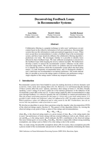
Figure 4: (Left to Right) A density plot of deconvolved and observed ratings on the Jester joke dataset(Left) that had no feedback loops and on the Netflix dataset (Left Center) where their Cinematchalgorithm was running. The Netflix data shows dispersive effects indicative of a RS whereas theJester data is highly correlated indicating no feedback system. A scatter plot of deconvolved andobserved ratings on the MusicLab dataset- Weak (Right Center) that had no downloads counts and onthe MusicLab dataset- Strong (Right) which displayed the download counts. The MusicLab-Strongscatter plot shows higher dispersive effects indicative of feedback effects.Datasets. Table 1 lists all the datasets we use to validate our approach for deconvolving a RS(from [21, 4, 13]). The columns detail name of the dataset, number of users, the number of items,the lower threshold for number of ratings per item (RPI) considered in the input ratings matrix andthe number of singular vectors k (as many as possible based on the limits of computer memory),respectively. The datasets are briefly discussed in the supplementary material.Classification of ratings matrix.An example of the types of insights our method enables is shown in Figure 4. This figure shows fourdensity plots of the estimated true ratings (y-axis) compared with the observed ratings (x-axis) fortwo datasets, Jester and Netflix. Higher density is indicated by darker shades in the scatter plot ofobserved and deconvolved ratings. If there is no RS, then these should be highly correlated. If thereis a system with feedback loops, we should see a dispersive plot. In the first plot (Jester) we see theresults for a real-world system without any RS or feedback loops; the second plot (Netflix) shows theresults on the Netflix ratings matrix, which did have a RS impacting the data. A similar phenomenonis observed in the third and fourth plots corresponding to the MusicLab dataset in Figure 4. Wedisplay the density plot of observed (y-axis) vs. deconvolved or expected true (x-axis) ratings for alldatasets considered in our evaluation in the supplementary material.Recommender system scores. The RS scores we displayedin Table 1 are based on the fraction of ratings with non-zeroscore (using the score metric (10)). Recall that a zero scoreindicates that the data point lies outside the associated hyperbola and does not suffer from recommender effect. Hence,the RS score is indicative of the fraction of ratings affectedby the recommender. Looking at Table 1, we see that the twoJester datasets have low RS scores validating that the Jesterdataset did not run a RS. The MusicLab datasets show a weakeffect because they do not include any type of item-item recommender. Nevertheless, the strong social influence conditionscored higher for a RS because the simple download countfeedback will elicit comparable effects. These cases give usconfidence in our scores because we have a clear understanding of feedback processes in the true data. Interestingly, theRS score progressively increases for the three versions of the Figure 5: (Top to bottom) (a) DeMovieLens datasets: MovieLens-100K, MovieLens-1M and convolved ranking as a bar chart forMovieLens-10M. This is expected as the RS effects would T.V. shows. (b) Deconvolved rankhave progressively accrued over time in these datasets. Note ing as a bar chart for Indian movies.that Netflix is also lower than Movielens, indicating that Netflix’s recommender likely correlated better with users’ true tastes. The RS scores associated withalcohol datasets (RateBeer, BeerAdvocate and Wine Ratings) are higher compared to the Fine Foodsdataset. This is surprising. We conjecture that this effect is due to common features that correlatewith evaluations of alcohol such as the age of wine or percentage of alcohol in beer.Ranking of items based on recommendation score. We associate a RS rating to each item as ourmean score of an item over all users. All items are ranked in ascending order of RS score and we7
first look at items with low RS scores. The Netflix dataset comprises of movies as well as televisionshows. We expect that television shows are less likely to be affected by a RS because each season ofa T.V. show requires longer time commitment, and they have their own following. To validate thisexpectation, we first identify all T.V. shows in the ranked list and compute the number of occurrencesof a T.V. show in equally spaced bins of size 840. Figure 5 shows a bar chart for the number ofoccurrences and we see that there are 90 T.V.shows in the first bin (or top 840 items as per thescore). This is highest compared to all bins and the number of occurrences progressively decreaseas we move further down the list, validating our expectation. Also unsurprisingly, the seasons ofthe popular sitcom Friends comprised of 10 out of the top 20 T.V. seasons with lowest RS scores.It is also expected that the Season 1 of a T.V. show is more likely to be recommended relative tosubsequent seasons. We identified the top 40 T.V shows with multiple (at least 2) seasons, andobserved that 31 of these have a higher RS score for Season 1 relative to Season 2. The 9 T.V. showswhere the converse is true are mostly comedies like Coupling, That 70’s Show etc., for which theseasons can be viewed independently of each other. Next, we looked at items with high RS score. Atthe time the dataset was released, Netflix operated exclusively in the U.S., and one plausible use isthat immigrants might use Netflix’s RS to watch movies from their native country. We specificallylooked at Indian films in the ranked list to validate this expectation. Figure 5b shows a bar chartsimilar to the one plotted for T.V. shows and we observe an increasing trend along the ranked list forthe number of occurrences of Indian films. The movie with lowest recommendation score is Lagaan,the only Indian movie to be nominated for the Oscars in last 25 years.4Discussion, related work and future workDiscussion:In this paper we propose a mechanism to deconvolve feedback effects on RS, similar inspirit to the network deconvolution method to distinguish direct dependencies in biological networks[10, 3]. Indeed, our approach can be viewed as a generalization of their methods for generalrectangular matrices. We do so by only considering a ratings matrix at a given instant of time. Ourapproach depends on a few reasonable assumptions that enable us to create a tractable model of a RS.When we evaluate the resulting methods on synthetic and real-world datasets, we find that we areable to assess the degree of influence that a RS has had on those ratings. This analysis is also easy tocompute and just involves a singular value decomposition of the ratings matrix.Related Work: User feedback in collaborative filtering systems is categorized as either explicitfeedback which includes input by users regarding their interest in products [1], or implicit feedbacksuch as purchase and browsing history, search patterns, etc. [14]. Both types of feedback affectthe item-item or user-user similarities used in the collaborative filtering algorithm for predictingfuture recommendations [16]. There has been a considerable amount of work on incorporating theinformation from these types of user feedback mechanisms in collaborative filtering algorithms inorder to improve and personalize recommendations [15, 6]. Here, we do not focus on improvingcollaborative filtering algorithms for recommender systems by studying user feedback, but instead,our thrust is to recover each user’s true preference of an item devoid of any rating bias introducedby the recommender system due to feedback. Another line of work based on user feedback inrecommender systems is related to understanding the exploration and exploitation tradeoff [20]associated with the training feedback loop in collaborative filtering algorithms [9]. This line ofresearch evaluates ‘what-if’ scenarios such as evaluating the performance of alternative collaborativefiltering models or, adapting the algorithm based on user-click feedbacks to maximize reward, usingapproaches like the multi-armed bandit setting [17, 18] or counterfactual learning systems [5]. Incontrast, we tackle the problem of recovering the true ratings matrix if feedback loops were absent.Future Work: In the future we wish to analyze the effect of feeding the derived deconvolved ratingswithout putative feedback effects back into the RS. Some derivatives of our method include settingthe parameters considered unknown in our current approach with known values (such as S ) if knowna priori. Incorporating temporal information at different snapshots of time while deconvolving thefeedback loops is also an
Feedback loop in RS wherein the observed ratings is a function of the true ratings and ratings induced by a RS 2.1 A model recommender system Consider a ratings matrix R of dimen-sion m n where m is the number of users and n is the number of items being rated. Users are denoted by subscript u, and items are denoted by subscript i, i.e., R