Transcription
Chapter 1Foundations of Engineering Economy1-1 IntroductionThe need for engineering economy is primarily motivated by the work that engineers doin performing analyses, synthesizing, and coming to a conclusion as they work onprojects of all sizes. In other words, engineering economy is at the heart of makingdecisions. These decisions involve the fundamental elements of cash flows of money,time, and interest rates. This chapter introduces the basic concepts and terminologynecessary for an engineer to combine these three essential elements in organized,mathematically correct ways to solve problems that will lead to better decisions.1-2 Why Engineering Economy and the Time Value of Money areImportantDecisions are made routinely to choose one alternative over another by engineers on thejob; by managers who supervise the activities of others; by corporate presidents whooperate a business; and by government officials who work for the public good. Mostdecisions involve money, called capital or capital funds, which is usually limited inamount. The decision of where and how to invest this limited capital is motivated by aprimary goal of adding value as future, anticipated results of the selected alternative arerealized. Engineers play a vital role in capital investment decisions based upon theirability and experience to design, analyze, and synthesize. The factors upon which adecision is based are commonly a combination of economic and noneconomic elements.Engineering economy deals with the economic factors. By definition,Engineering economy involves formulating, estimating, and evaluating the expectedeconomic outcomes of alternatives designed to accomplish a defined purpose.Mathematical techniques simplify the economic evaluation of alternatives.Because the formulas and techniques used in engineering economics are applicable toall types of money matters, they are equally useful in business and government, as wellas for individuals.1
To be financially literate is very important as an engineer and as a person. Unfortunatelymany people do not have the fundamental understanding of concepts such as financialrisk and diversification, inflation, numeracy, and compound interest. You will learn andapply these basic concepts, and more, through the study of engineering economyOther terms that mean the same as engineering economy are engineering economicanalysis, capital allocation study, economic analysis, and similar descriptors.People make decisions; computers, mathematics, concepts, and guidelines assist peoplein their decision-making process. Since most decisions affect what will be done, the timeframe of engineering economy is primarily the future. Therefore, the numbers used inengineering economy are best estimates of what is expected to occur. The estimatesand the decision usually involve four essential elements:Cash flowsTimes of occurrence of cash flowsInterest rates for time value of moneyMeasure of worth for selecting an alternativeSince the estimates of cash flow amounts and timing are about the future, they will besomewhat different than what is actually observed, due to changing circumstances andunplanned events. In short, the variation between an amount or time estimated now andthat observed in the future is caused by the stochastic (random) nature of all economicevents. Sensitivity analysis is utilized to determine how a decision might changeaccording to varying estimates, especially those expected to vary widely.The criterion used to select an alternative in engineering economy for a specific set ofestimates is called a measure of worth. The measures developed and used in this textarePresent worth (PW)Future worth (FW)Annual worth (AW)Rate of return (ROR)Benefit/cost (B/C)Capitalized cost (CC)Payback periodProfitability indexEconomic value added (EVA)All these measures of worth account for the fact that money makes money over time.This is the concept of the time value of money.2
It is a well-known fact that money makes money. The time value of money explains thechange in the amount of money over time for funds that are owned (invested) or owed(borrowed). This is the most important concept in engineering economy.The time value of money is very obvious in the world of economics. If we decide toinvest capital (money) in a project today, we inherently expect to have more money inthe future than we invested. If we borrow money today, in one form or another, weexpect to return the original amount plus some additional amount of money. Anengineering economic analysis can be performed on future estimated amounts or on pastcash flows to determine if a specific measure of worth, e.g., rate of return, was achieved.Engineering economics is applied in an extremely wide variety of situations. Samplesare: Equipment purchases and leases Chemical processes Cyber security Construction projects Airport design and operations Sales and marketing projects Transportation systems of all types Product design Wireless and remote communication and control Manufacturing processes Safety systems Hospital and healthcare operations Quality assurance Government services for residents and businessesIn short, any activity that has money associated with it—which is just about everything—is a reasonable topic for an engineering economy study.EXAMPLE 1.1Cyber security is an increasingly costly dimension of doing business for many retailersand their customers who use credit and debit cards. A 2014 data breach of U.S.-based3
Home Depot involved some 56 million cardholders. Just to investigate and cover theimmediate direct costs of this identity theft amounted to an estimated 62,000,000, ofwhich 27,000,000 was recovered by insurance company payments. This does notinclude indirect costs, such as, lost future business, costs to banks, and cost to replacecards. If a cyber security vendor had proposed in 2006 that a 10,000,000 investment ina malware detection system could guard the company's computer and payment systemsfrom such a breach, would it have kept up with the rate of inflation estimated at 4% peryear?SolutionAs a result of this data breach, Home Depot experienced a direct out-of-pocket cost of 35,000,000 after insurance payments. From learning to the engineering economy, youwill learn how to determine the future equivalent of money at a specific rate. In this case,the estimate of 10,000,000 after 8 years (from 2006 to 2014) at an inflation rate of 4%is equivalent to 13,686,000.The 2014 equivalent cost of 13.686 million is significantly less than the out-of-pocketloss of 35 million. The conclusion is that the company should have spent 10 millionin 2006.Besides, there may be future breaches that the installed system will detect and eliminate.This is an extremely simple analysis; yet, it demonstrates that at a very elementary level,it is possible to determine whether an expenditure at one point in time is economicallyworthwhile at some time in the future. In this situation, we validated that a previousexpenditure (malware detection system) should have been made to overcome anunexpected expenditure (cost of the data breach) at a current time, 2014 here.1.3 Performing an Engineering Economy StudyAn engineering economy study involves many elements: problem identification,definition of the objective, cash flow estimation, financial analysis, and decisionmaking. Implementing a structured procedure is the best approach to select the bestsolution to the problem.The steps in an engineering economy study are as follows:1. Identify and understand the problem; identify the objective of the project.2. Collect relevant, available data and define viable solution alternatives.4
3. Make realistic cash flow estimates.4. Identify an economic measure of worth criterion for decision making.5. Evaluate each alternative; consider noneconomic factors; use sensitivity analysis asneeded.6. Select the best alternative.7. Implement the solution and monitor the results.Technically, the last step is not part of the economy study, but it is, of course, a stepneeded to meet the project objective.5
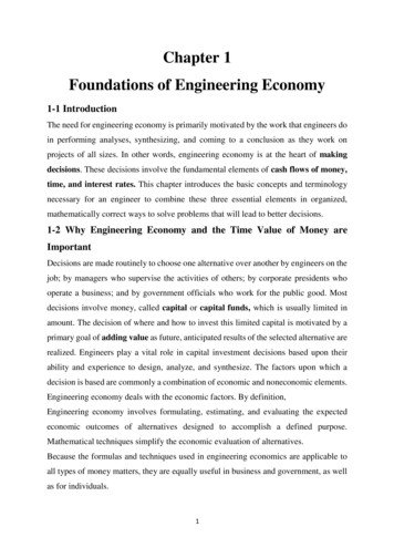
Fig. 1 Steps in an engineering economy study.1.4 Interest Rate and Rate of ReturnInterest is the manifestation of the time value of money. Computationally, interest is thedifference between an ending amount of money and the beginning amount. If thedifference is zero or negative, there is no interest. There are always two perspectives toan amount of interest—interest paid and interest earned. These are illustrated in Fig.2.6
Interest is paid when a person or organization borrowed money (obtained a loan) andrepays a larger amount over time. Interest is earned when a person or organization saved,invested, or lent money and obtains a return of a larger amount over time. The numericalvalues and formulas used are the same for both perspectives, but the interpretations aredifferent.Interest paid on borrowed funds (a loan) is determined using the original amount, alsocalled the principal,Interest amount owed now principal(1)When interest paid over a specific time unit is expressed as a percentage of the principal,the result is called the interest rate.Interest rate (%) ܑ ܜܑܖܝ ܍ ܕܑܜ ܚ܍ܘ ܌ܚܚ܋ܝ܋܉ ܜܛ܍ܚ܍ܜܖ 100%(2)The time unit of the rate is called the interest period. By far the most common interestperiod used to state an interest rate is 1 year. Shorter time periods can be used, such as1% per month.Thus, the interest period of the interest rate should always be included. If only the rateis stated, for example, 8.5%, a 1-year interest period is assumed.Fig. 1–2 (a) Interest paid over time to lender. (b) Interest earned over time byinvestor.EXAMPLE 1.2An employee at LaserKinetics.com borrows 10,000 on May 1 and must repay a totalof 10,700 exactly 1 year later. Determine the interest amount and the interest rate paid.SolutionThe perspective here is that of the borrower since 10,700 repays a loan. Apply Equation7
Interest amount owed now principalTo determine the interest paid.Interest paid 10,700 10,000 700Then determine the interest rate paid for 1 year.Interest rate (%) Percent Interest rate (%) EXAMPLE 1.3 ଵ ܑ ܜܑܖܝ ܍ ܕܑܜ ܚ܍ܘ ܌ܚܚ܋ܝ܋܉ ܜܛ܍ܚ܍ܜܖ 100% 7% per year 100%Stereophonics, Inc. plans to borrow 20,000 from a bank for 1 year at 9% interest fornew recording equipment. (a) Compute the interest and the total amount due after 1 year.(b) Construct a column graph that shows the original loan amount and total amount dueafter 1 year used to compute the loan interest rate of 9% per year.Solution(a) Compute the total interest accrued by solving Equation [2] for interest accrued.Interest 20,000(0.09) 1800The total amount due is the sum of principal and interest.Total due 20,000 1800 21,800(b) Figure 3 shows the values used in Equation [2]: 1800 interest, 20,000 original loanprincipal, 1-year interest period.Fig. 3 Values used to compute an interest rate of 9% per year. Example 1.3.8
CommentNote that in part (a), the total amount due may also be computed asTotal due principal (1 interest rate) 20,000(1.09) 21,800Later we will use this method to determine future amounts for times longer than oneinterest period.From the perspective of a saver, a lender, or an investor, interest earned (Fig.2b) is thefinal amount minus the initial amount, or principal.Interest earned total amount now principal(3)Interest earned over a specific period of time is expressed as a percentage of the originalamount and is called rate of return (ROR). ܖܚܝܜ܍ܚ ܗ ܍ܜ܉ܚ ۷ ܜܛ܍ܚ܍ܜܖ %(4)The time unit for rate of return is called the interest period, just as for the borrower’s perspective.Again, the most common period is 1 year.The term return on investment (ROI) is used equivalently with ROR in differentindustries and settings, especially where large capital funds are committed toengineering-oriented programs.The numerical values in Equations [2] and [4] are the same, but the term interest ratepaid is more appropriate for the borrower's perspective, while the term rate of returnearned applies for the investor's perspective.EXAMPLE 1.5(a) Calculate the amount deposited 1 year ago to have 1000 now at an interest rate of5% per year.(b) Calculate the amount of interest earned during this time period.Solution(a) The total amount accrued ( 1000) is the sum of the original deposit and the earnedinterest.If X is the original deposit,Total accrued deposit deposit (interest rate) 1000 X X (0.05) X (1 0.05) 1.05XThe original deposit is9
ܺ 1000 952.381.05(b) Apply Equation [3] to determine the interest earned.Interest 1000 952.38 47.621.5 Terminology and SymbolsThe equations and procedures of engineering economy utilize the following terms andsymbols.Sample units are indicated.P value or amount of money at a time designated as the present or time 0. Also P isreferred to as present worth (PW), present value (PV), net present value (NPV),discounted cash flow (DCF), and capitalized cost (CC); monetary units, such as dollarsF value or amount of money at some future time. Also F is called future worth (FW)and future value (FV); dollarsA series of consecutive, equal, end-of-period amounts of money. Also A is called theannual worth (AW) and equivalent uniform annual worth (EUAW); dollars per year,euros per monthn number of interest periods; years, months, daysi interest rate per time period; percent per year, percent per montht time, stated in periods; years, months, daysThe symbols P and F represent one-time occurrences: A occurs with the same value ineach interest period for a specified number of periods. It should be clear that a presentvalue P represents a single sum of money at some time prior to a future value F or priorto the first occurrence of an equivalent series amount A.It is important to note that the symbol A always represents a uniform amount (i.e., thesame amount each period) that extends through consecutive interest periods. Bothconditions must exist before the series can be represented by A.The interest rate i is expressed in percent per interest period, for example, 12% per year.Unless stated otherwise, assume that the rate applies throughout the entire n years orinterest periods.The decimal equivalent for i is always used in formulas and equations in engineeringeconomy computations.10
All engineering economy problems involve the element of time expressed as n andinterest rate i. In general, every problem will involve at least four of the symbols P, F,A, n, and i, with at least three of them estimated or known.EXAMPLE 1.6Last year Jane’s grandmother offered to put enough money into a savings account togenerate 5000 in interest this year to help pay Jane’s expenses at college. (a) Identifythe symbols, and (b) calculate the amount that had to be deposited exactly 1 year ago toearn 5000 in interest now, if the rate of return is 6% per year.Solution(a) Symbols P (last year is -1) and F (this year) are needed.P ?i 6% per yearn 1 yearF P interest ? 5000(b) Let F total amount now and P original amount. We know that F – P 5000 isaccrued interest. Now we can determine P. Refer to Equations [1] through [4].F P PiThe 5000 interest can be expressed asInterest F – P (P Pi) – P Pi 5000 P (0.06)1.6 Cash Flows: Estimation and DiagrammingAs mentioned in earlier sections, cash flows are the amounts of money estimated forfuture projects or observed for project events that have taken place. All cash flows occurduring specific time periods, such as 1 month, every 6 months, or 1 year. Annual is themost common time period. For example, a payment of 10,000 once every year inDecember for 5 years is a series of 5 outgoing cash flows. And an estimated receipt of 500 every month for 2 years is a series of 24 incoming cash flows. Engineeringeconomy bases its computations on the timing, size, and direction of cash flows.11
Cash inflows are the receipts, revenues, incomes, and savings generated by project andbusiness activity. A plus sign indicates a cash inflow.Cash outflows are costs, disbursements, expenses, and taxes caused by projects andbusiness Cash flow activity. A negative or minus sign indicates a cash outflow. Whena project involves only costs, the minus sign may be omitted for some techniques, suchas benefit/cost analysis.Some examples of cash flow estimates are shown here. As you scan these, consider howthe cash inflow or outflow may be estimated most accurately.Cash Inflow EstimatesIncome: 150,000 per year from sales of solar-powered watchesSavings: 24,500 tax savings from capital loss on equipment salvageReceipt: 750,000 received on large business loan plus accrued interestSavings: 150,000 per year saved by installing more efficient air conditioningRevenue: 50,000 to 75,000 per month in sales for extended battery life iPhonesCash Outflow EstimatesOperating costs: 230,000 per year annual operating costs for software servicesFirst cost: 800,000 next year to purchase replacement earthmoving equipmentExpense: 20,000 per year for loan interest payment to bankInitial cost: 1 to 1.2 million in capital expenditures for a water recycling unitAll of these are point estimates, that is, single-value estimates for cash flow elementsof an alternative, except for the last revenue and cost estimates listed above. Theyprovide a range estimate, because the persons estimating the revenue and cost do nothave enough knowledge or experience with the systems to be more accurate. For theinitial chapters, we will utilize point estimates. Once all cash inflows and outflows areestimated (or determined for a completed project), the net cash flow for each time periodis calculated.Net cash flow cash inflows - cash outflows(5)NCF R - D(6)Where NCF is net cash flow, R is receipts, and D is disbursementsAt the beginning of this section, the timing, size, and direction of cash flows werementioned as important. Because cash flows may take place at any time during an12
interest period, as a matter of convention, all cash flows are assumed to occur at the endof an interest period.The cash flow diagram is a very important tool in an economic analysis, especiallywhen the cash flow series is complex. It is a graphical representation of cash flows drawnon the y axis with a time scale on the x axis. The diagram includes what is known, whatis estimated, and what is needed. That is, once the cash flow diagram is complete,another person should be able to work the problem by looking at the diagram.Cash flow diagram time t 0 is the present, and t 1 is the end of time period 1. Weassume that the periods are in years for now. The time scale of Fig.4 is set up for 5 years.Since the end-of-year convention places cash flows at the ends of years, the “1” marksthe end of year 1.While it is not necessary to use an exact scale on the cash flow diagram, you willprobably avoid errors if you make a neat diagram to approximate scale for both time andrelative cash flow magnitudes.The direction of the arrows on the diagram is important to differentiate income fromoutgo. A vertical arrow pointing up indicates a positive cash flow. Conversely, a downpointing arrow indicates a negative cash flow. We will use a bold, colored arrow toindicate what is unknown and to be determined.For example, if a future value F is to be determined in year 5, a wide, colored arrowwith F ? is shown in year 5. The interest rate is also indicated on the diagram.Figure 5 illustrates a cash inflow at the end of year 1, equal cash outflows at the end ofyears 2 and 3, an interest rate of 4% per year, and the unknown future value F after 5years. The arrow for the unknown value is generally drawn in the opposite directionfrom the other cash flows; however, the engineering economy computations willdetermine the actual sign on the F value.Fig. 4 A typical cash flow time scale for 5 years.13
Fig. 5 Example of positive and negative cash flows.Before the diagramming of cash flows, a perspective or vantage point must bedetermined so that or – signs can be assigned and the economic analysis performedcorrectly. Assume you borrow 8500 from a bank today to purchase an 8000 used carfor cash next week, and you plan to spend the remaining 500 on a new paint job for thecar two weeks from now. There are several perspectives possible when developing thecash flow diagram—those of the borrower (that’s you), the banker, the car dealer, or thepaint shop owner. The cash flow signs and amounts for these perspectives are as follows.Fig. 6 Cash flows from perspective of borrower for loan and purchases.14
EXAMPLE 1.7Each year Exxon-Mobil expends large amounts of funds for mechanical safety featuresthroughout its worldwide operations. Carla Ramos, a lead engineer for Mexico andCentral American operations, plans expenditures of 1 million now and each of the next4 years just for the improvement of field-based pressure-release valves. Construct thecash flow diagram to find the equivalent value of these expenditures at the end of year4, using a cost of capital estimate for safety-related funds of 12% per year.SolutionFigure 7 indicates the uniform and negative cash flow series (expenditures) for fiveperiods, and the unknown F value (positive cash flow equivalent) at exactly the sametime as the fifth expenditure. Since the expenditures start immediately, the first 1million is shown at time 0, not time 1. Therefore, the last negative cash flow occurs atthe end of the fourth year, when F also occurs. To make this diagram have a full 5 yearson the time scale, the addition of the year -1 completes the diagram. This additiondemonstrates that year 0 is the end-of-period point for the year 1.Fig. 7 Cash flow diagramEXAMPLE 1.8An electrical engineer wants to deposit an amount P now such that she can withdraw anequal annual amount of A1 2000 per year for the first 5 years, starting 1 year after thedeposit, and a different annual withdrawal of A2 3000 per year for the following 3years. How would the cash flow diagram appear if i 8.5% per year?SolutionThe cash flows are shown in Fig. 8. The negative cash outflow P occurs now. Thewithdrawals (positive cash inflow) for the A1 series occur at the end of years 1 through5, and A2 occurs in years 6 through 8.15
Fig. 8 Cash flow diagram with two different A series.EXAMPLE 1.9A rental company spent 2500 on a new air compressor 7 years ago. The annual rentalincome from the compressor has been 750. The 100 spent on maintenance the firstyear has increased each year by 25. The company plans to sell the compressor at theend of next year for 150. Construct the cash flow diagram from the company’sperspective and indicate where the present worth now is located.SolutionLet now be time t 0. The incomes and costs for years -7 through 1 (next year) aretabulated below with net cash flow computed using Equation (5). The net cash flows(one negative, eight positive) are diagrammed in Fig. 9. Present worth P is located atyear 0.16
Fig. 9 Cash flow diagram.1.7 Economic EquivalenceEconomic equivalence is a fundamental concept upon which engineering economycomputations are based.Economic equivalence is a combination of interest rate and time value of money todetermine the different amounts of money at different points in time that are equal ineconomic value.As an illustration, if the interest rate is 6% per year, 100 today (present time) isequivalent to 106 one year from today.Amount accrued 100 100(0.06) 100(1 0.06) 106In addition to future equivalence, we can apply the same logic to determine equivalencefor previous years. A total of 100 now is equivalent to 100 1.06 94.34 one yearago at an interest rate of 6% per year. From these illustrations, we can state thefollowing: 94.34 last year, 100 now, and 106 one year from now are equivalent atan interest rate of 6% per year. The fact that these sums are equivalent can be verifiedby computing the two interest rates for 1-year interest periods.The cash flow diagram in Fig.10 indicates the amount of interest needed each year tomake these three different amounts equivalent at 6% per year.17
Fig. 10 Equivalence of money at 6% per year interest.1.8 Simple and Compound InterestThe terms interest, interest period, and interest rate (introduced in Section 1.4) areuseful in calculating equivalent sums of money for one interest period in the past andone period in the future. However, for more than one interest period, the terms simpleinterest and compound interest become important.Simple interest is calculated using the principal only, ignoring any interest accrued inpreceding interest periods. The total simple interest over several periods is computed asSimple interest (principal) (number of periods) (interest rate)(7)I PniWhere I is the amount of interest earned or paid and the interest rate i is expressed indecimal form.EXAMPLE 1.10GreenTree Financing lent an engineering company 100,000 to retrofit anenvironmentally unfriendly building. The loan is for 3 years at 10% per year simpleinterest. How much money will the firm repay at the end of 3 years?SolutionThe interest for each of the 3 years isInterest per year 100,000(0.10) 10,000Total interest for 3 years from Equation (7) is18
Total interest 100,000(3) (0.10) 30,000The amount due after 3 years isTotal due 100,000 30,000 130,000The interest accrued in the first year and in the second year does not earn interest. Theinterest due each year is 10,000 calculated only on the 100,000 loan principal.In most financial and economic analyses, we use compound interest calculations.For compound interest, the interest accrued for each interest period is calculated on thePrincipal plus the total amount of interest accumulated in all previous periods.Thus, compound interest means interest on top of interest. Compound interest reflectsthe effect of the time value of money on the interest also. Now the interest for one periodis calculated asCompound interest (principal all accrued interest) (interest rate)(8)In mathematical terms, the interest It for time period t may be calculated using therelation.(9)EXAMPLE 1.11Assume an engineering company borrows 100,000 at 10% per year compound interestand will pay the principal and all the interest after 3 years. Compute the annual interestand total amount due after 3 years. Graph the interest and total owed for each year, andcompare with the previous example that involved simple interest.SolutionTo include compounding of interest, the annual interest and total owed each year arecalculated by Equation (8).Interest, year 1: 100,000(0.10) 10,000Total due, year 1: 100,000 10,000 110,000Interest, year 2: 110,000(0.10) 11,000Total due, year 2: 110,000 11,000 121,000Interest, year 3: 121,000(0.10) 12,100Total due, year 3: 121,000 12,100 133,10019
The repayment plan requires no payment until year 3 when all interest and the principal,a total of 133,100, are due. Figure 1–11 uses a cash flow diagram format to compareend-of-year (a) simple and (b) compound interest and total amounts owed. Thedifferences due to compounding are clear. An extra 133,100 – 130,000 3100 ininterest is due for the compounded interest loan.Note that while simple interest due each year is constant, the compounded interest duegrows geometrically. Due to this geometric growth of compound interest, the differencebetween simple and compound interest accumulation increases rapidly as the time frameincreases.For example, if the loan is for 10 years, not 3, the extra paid for compounding interestmay be calculated to be 59,374.Fig.11 Interest I owed and total amount owed for (a) simple interest (Example 1.10) and(b) compound interest (Example 1.11).A more efficient way to calculate the total amount due after a number of years inExample 1.11 is to utilize the fact that compound interest increases geometrically. Thisallows us to skip the year by year computation of interest. In this case, the total amountdue at the end of each year is20
Year 1: 100,000(1.10)1 110,000Year 2: 100,000(1.10)2 121,000Year 3: 100,000(1.10)3 133,100This allows future totals owed to be calculated directly without intermediate steps. Thegeneral form of the equation isTotal due after n years principal (1 interest rate) n years(10) P (1 i) nWhere i is expressed in decimal form. The total due after n years is the same as the futureworth F, defined in Section 1.5. Equation (10) was applied above to obtain the 133,100due after 3 years. This fundamental relation will be used many times in the upcomingchapters.We can combine the concepts of interest rate, compound interest, and equivalence todemonstrate that different loan repayment plans may be equivalent, but differsubstantially in amounts paid from one year to another and in the total repaymentamount. This also shows that there are many ways to take into account the time value ofmoney.EXAMPLE 1.12Table 1–1 details four different loan repayment plans described below. Each plan repaysa 5000 loan in 5 years at 8% per year compound interest. Plan 1: Pay all at end. No interest or principal is paid until the end of year 5. Interestaccumulates each year on the total of principal and all accrued interest. Plan 2: Pay interest annually, principal repaid at end. The accrued interest ispaid each year, and the entire principal is repaid at the end of year 5. Plan 3: Pay interest and portion of principal annually. The accrued interest andone-fifth of the principal (or 1000) are repaid each year. The outstanding loanbalance decreases each year, so the interest (column 2) for each year decreases. Plan 4: Pay equal amount of interest and principal. Equal payments are madeeach year with a portion going toward principal repayment and
Implement the solution and monitor the results. Technically, the last step is not part of the economy study, but it is, of course, a step needed to meet the project objective. 6 Fig. 1 Steps in an engineering economy study. 1.4 Interest Rate and Rate of Return