Transcription
Proceedings of the46th IEEE Conference on Decision and ControlNew Orleans, LA, USA, Dec. 12-14, 2007FrA12.2Using distributed magnetometers to increase IMU-based velocityestimation into perturbed areaDavid Vissière, Alain Martin, Nicolas PetitAbstract— We address the problem of position estimation fora rigid body using an inertial measurement unit (IMU) and a setof spatially distributed magnetometers. We take advantage ofthe magnetic field disturbances usually observed indoors. Thisis particularly relevant when GPS is unavailable (e.g. duringmilitary operations in urban areas). We illustrate our techniquewith several experimental results obtained with a Kalman filter.We also present our testing bench which consists of low costsensors (IMU and magnetometers).I NTRODUCTIONNumerous military and civilian control applications require high accuracy position, speed, and attitude estimations of a solid body. Examples range from UnmannedAir Vehicles (UAV), Unmanned Ground Vehicles (UGV),full-sized submarines, sub-sea civil engineering positioningdevices [10], to name a few. A widely considered solutionis to use embedded Inertial Measurement Units (IMU).Accelerometers, gyroscopes (and possibly magnetometers)signals can be used to derive position information througha double integration process [5], [4]. Because of sensorsdrifts, this approach requires very high precision IMUs Othersolutions need to be used when cost, space, or weightconstraints become stringent. A recent trend has been toheavily rely on the well known Global Positioning system(GPS) technology. has a limited availability (especially inthe context of military operations), its accuracy is (roughlyspeaking) of 10 m of error. GPS is very poorly useablebetween buildings in forests or indoor. The recent progressin very low cost (less than 1,500 USD), low weight (lessthan 100 g) and low size (less than 3 cm2 ) IMUs havespurred a broad interest in the development of IMU-basedpositioning technologies. These Micro-Electro-MechanicalSystems (MEMS) IMUs appear to have quickly increasingcapabilities. Several manufacturers are announcing new models under 5,000 USD with gyroscopes capable of less than20 deg/hr.So far, there does not exist any reported experiment ofsuccessful position estimation from such a low cost IMU.In the literature, these IMUs are only used for attitudeestimation (see e.g. [3], [7] or [2] for an application to thecontrol of mini-UAVs in closed loop). Some tentative workD. Vissière (corresponding author) is “Ingénieur de l’Armement” in theDélégation Générale pour l’Armement (DGA) of the French Departmentof Defense. He is a PhD candidate in Mathematics and Control, CentreAutomatique et Systèmes, École des Mines de Paris, 60, bd St Michel, 75272Paris, France david.vissiere@dga.defense.gouv.frA. Martin is “Ingénieur” in the Délégation Générale pour l’Armement(DGA) of the French Department of Defense.N. Petit is with the Centre Automatique et Systèmes, École NationaleSupérieure des Mines de Paris, 60, bd St Michel, 75272 Paris, France1-4244-1498-9/07/ 25.00 2007 IEEE.Fig. 1. A typical platoon of soldiers in action as envisioned in the BOAprojet. c F.Blanchard-BD Médias for Délégation Générale pour l’Armement(DGA). A team leader keeps track of his soldiers thanks to real-time positioninformation reported on his arm held display.(using higher-end IMUs) address the problem of velocitiesestimation. In these cases, the speed information is obtainedfrom a GPS receiver using the Doppler effect (see [5] fordetails on the quality of the obtained measurements information) or from odometers (in the case of ground vehicles).Our focus is on indoor missions involving humans. It isdesired to remotely estimate their positions. During preliminary tests, it quickly appeared to us that, given the poorknowledge of the body dynamics, it is impossible to geta position error below 50 m from a low cost IMU (e.g.a 3DMGX1 from Microstrainr) after a few minutes ofexperiments. For the specific problem of pedestrian indoornavigation, technical solutions exist in both academia [8],and industry (e.g. Core Navigation Module by Vectronixr).These methods do not rely on velocity inertial estimates,but, rather, evaluate step lengths and walking pace. AnIMU is used to provide heading information, and to detectstop and go sequences. Obtained results are good, providedthat the pedestrian is not walking side ways, and keeps aregular step length. It is also required that the magneticfield is not disturbed. High-end IMUs are usually muchtoo heavy for human-oriented applications. While the GPSsignal is poorly available indoor, experimental measurementshave shown that the magnetic field in a typical businessbuilding is strongly disturbed (by the building structure,electrical equipments and computers among others). For sakeof illustration, we report the variations of the magnetic fieldnorm inside a business building office in Figure 2.Our claim is that these disturbances (which are assumed to4924
46th IEEE CDC, New Orleans, USA, Dec. 12-14, 2007the measurement equations from available sensors (namelygyroscopes, accelerometers and 12.20200400600800time (s)1000120014001600Fig. 2. Variation of the magnetic field norm during a 2.4 m horizontaldisplacement inside a business building office.be stationary) can actually be used to improve the positionestimation. Our work is related to the approach advocatedin [6] for gravimetry aided navigation. Very importantly, ourapproach does not rely on any a-priori magnetic map. Itsimply uses Maxwell’s equation. In words, we note that, ina disturbed magnetic field, it is possible to determine whena solid body equipped with 4 magnetometers is moving. If itmoves, then the sensed magnetic fields must change in accordance with Maxwell’s law. If the magnetic measurements donot change significantly, then the solid body is not moving.This allows us to rule out velocity drifts from the estimation.Eventually, this improves the position information obtainedby integrating the velocity estimate. In [11], we proposed,in a first approach, to model the magnetic field spatialderivatives with low pass dynamics driven by white noises.Here, we use an orthogonal trihedron of magnetometers, todirectly measure these derivatives and reconciliate magneticand inertial information. The experimental results that wepresent lead us to believe it is possible to estimate theposition of a man who is investing a building while bearinga low cost package consisting of an IMU and 3 additionalmagnetometers . This objective fits in the network centricwarfare (as defined in [9]) context “Bulle OpérationnelleAéroterrestre” (BOA), led by the Délégation Générale pourl’Armement (DGA) for the French Department of Defense.A typical mission in the BOA environment is depicted inFigure 1.The article is organized as follows. In Section I, we definethe position estimation problem. Notations required for thestudy of the dynamics are presented. In Section II, we exposeour use of magnetic disturbances and sensors. In particular,in that case, we prove the observability of the velocity. InSection III, we present experimental results, discuss implementation details, and comment on the calibration issues.Finally, in Section IV, we conclude and suggest severaldirections of improvement.I. P ROBLEM STATEMENTIn this section, we present the equation of motion ofa rigid body, the various frames under consideration, andA. Coordinate frames, system of equations, notationsAn IMU (viewed as a material point) is located at thecenter of gravity of a moving body we desire to estimatethe position of. This six degrees of freedom system cansimultaneously rotate and translate. A body-fixed referenceframe with origin at the center of gravity of the IMU isconsidered. In the following, subscript b refers to this bodyframe. The x, y and z axis are the IMU axis (i.e. areconsistent with the inner sensors orientations).As inertial reference frame, we consider the local frame.It corresponds to the North-East-Down frame when initialheading is zero: NED, the X axis is tangent to the geoid andis pointing to the north, the Z axis is pointing to the centerof the Earth, and the Y axis is tangent to the geoid and ispointing to the East. Subscript i refers to this inertial frame.The IMU delivers a 9 parameters vector [YV YΩ YM0 ]Tobtained from a 3-axis accelerometer, a 3-axis gyroscope anda 3-axis magnetometer. Measurements are noisy and biased.Classically, we consider that the accelerometer signal YVhas a bias BV (independently on each axis) and suffersfrom additive white noise µv R3 , and that both themagnetometer signal YM0 and the gyros signal YΩ haveadditive white noises µM R3 and µΩ R3 , respectively.Finally, there is a drift BΩ R3 on YΩ . It is possible toconsider unknown scale factors to increase filtering accuracy,but these are not necessary in a first approach. We noteBV R3 the drift of the accelerometer and BΩ R3 thedrift of the gyroscope.The rigid body is also equipped with three external magnetometers. These deliver three 3 measurement vectors[YM1 YM2 YM3 ]T . Each magnetometer has its own unknown scale factor, bias, and misalignment angles. To usethese signals, it is necessary to precisely obtain good estimates of these unknown parameters. A calibration procedureis presented in Section III.Noting F the external forces (excluding gravity) acting onthe IMU, and R the rotation matrix from the inertial frameto the body frame, we can write the measurement equationsfrom the IMU as Y [YV YΩ YM0 ]T with YV F R g BV µV YΩ Ω BΩ µΩ(1) YM0 M µM0where g stands for the gravity vector with norm g, and M isthe magnetic field in the body frame. For the bias vector B [BV BΩ ]T , several models can be considered dependingon accuracy requirements. A second order damped oscillatordriven by a white noise is a good choice. Classically, in filterequations, bias will be treated in an extended state.From a dynamical system point of view, the state of therigid body is described by the 12 following independentvariables.T X [x y z] is the position of the center of gravityof the IMU in the inertial frame4925
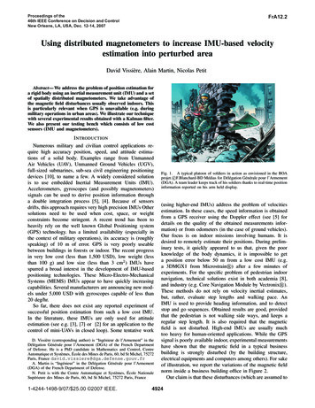
46th IEEE CDC, New Orleans, USA, Dec. 12-14, 2007FrA12.2TV [u v w] is the vector velocity of the center ofgravity of the IMU in the body frameT Q [φ θ ψ] stands for the Euler angles, i.e. theangles between the inertial frame and the bodyT Ω [p q r] are the angular rates.The input vector of the dynamics are the forces F T[Fu Fv Fw ] and torques. We call R the rotation matrixfrom the inertial frame to the body frame. cψcθsψcθ sθR cφsψ sφsθcψ cφcψ sφsψsθ cθsφ sφsψ cφsθcψ sφcψ cφsψsθ cθcφ with the notations c cos( ), s sin( ).Remark: To avoid the well known singularities when θreaches π2 , quaternions can be used to represent the Eulerangles. For sake of simplicity, we do not present quaternionsequations but they are handy in this situation, and useful toimplement the filter equations.B. Equations of motionThe matrix of inertia of the system is unknown. It isapproximated by the identity matrix. Models for the unknownforces F and angular rates Ω dynamics must be chosen.A very basic choice is to model them with white noises.Implicitly, the variance of the white noises νΩ and νF isused to specify the manoeuvring capabilities of our system.In summary, using the matrix R, we get the following systemdynamics Ẋ RT V V̇ Ω V F (2)Q̇ G(Ω, Q) Ω̇ νΩ Ḟ νFwith p (q sin(φ) r cos(φ)) tan(θ) q cos(φ) r sin(φ)G(Ω, Q) 1(q sin(φ) r cos(φ))cos(θ)II. U SING MAGNETIC FIELD DISTURBANCES TO OBSERVETHE VELOCITYNaturally, the measurements are expressed in the bodyframe. The magnetic field M is obtained through the relationM RMi(3)The usual way to take the magnetic measurements intoaccount in attitude or position estimation techniques is toconsider it gives a direct measure of the heading vector.This approach gives very good results, provided magneticdisturbances are negligible. Yet, as can be seen in Figure 2and Figure 3, these disturbances are not negligible indoor,e.g. in typical business offices or houses.In the inertial frame, the following three properties can bederived from Maxwell’s equations [1]. The magnetic field is stationary. According to Faraday’slaw of induction, in the absence of electrical sources0.6Mz discrethzx discret50.50.40.30.20.100. 10. 2050100150position along the wood rail (cm)200250Fig. 3. Histories of hzx the partial derivative of the z component of themagnetic field in the x inertial direction during a 2.1 m move at constantspeed along a wood (therefore non-magnetic) rail. Mi t 0. In other words, the magnetic field is afunction of the position only. We note it Mi (X). The magnetic field is a potential field. According toAmpère’s law, in the absence of electric and magneticsources, curl(Mi ) 0. Therefore, there exists a scalarfunction h(X) such that Mi h. The divergence of the magnetic field is zero: div(Mi ) 0. Thanks to the previous property, this implies h hxx hyy hzz 0.In the body frame, one can differentiate (3) to get thefollowing differential equation (thanks to a chain rule)Ṁ Ω M R 2 hRT V(4)In [11], we considered this equation by assuming that 2 hwas unknown and modeled its components by first order dynamics driven by white noises νH . We extended the state byadding the magnetic field M and the independent gradientsH. Due to the three properties presented above, there are onlyfive independent gradients to reconstruct. These are, in theTinertial frame, H , [hxx hxy hxz hyy hyz ] R5 .Some experiments have shown that strongly varying magnetic fields are difficult to estimate using this approach.In this paper, we use a set of magnetometers to evaluate 2 h. Three 3-axis magnetometers are precisely mountedon a board, see Figure 4. The exact locations are defined byvector lever arms l1 , l2 , and l3 which define a direct orthogonal trihedron. The sought after variables H are obtained fromfinite difference schemes. Further, we model their dynamicsby a white noiseḢ νH(5)Slopes depicted in Figure 3 suggest that spatial derivativesof H are not negligible. For sake of performance, it isrecommended to include some higher order dynamics in bothmeasurement and dynamics equations. For sake of simplicity,we do not present them here, but they can be easily takeninto account.Under the preceding assumptions, the vector of measurement obtained from the IMU, and the orthogonal trihedron4926
46th IEEE CDC, New Orleans, USA, Dec. 12-14, 2007of magnetometers is modeled asYV F Rg BV µVYΩ Ω BΩ µΩYM0 M µM0 YM1 M R 2 hRT l1 µM1 YM2 M R 2 hRT l2 µM2 2TYM3 M R hR l3 µM3(6)As will now appear, Equation (4) plays a key role inthis observation problem. It is the only one giving directinformation on V .A. Observability1) Linearization: In a general approach, let us considerthe system obtained by linearizing the dynamics (2)-(4)-(5),and the measurement Equation (6). We denote by X f thepartial derivative of f with respect to X, X f f x .From Equations (2)-(4)-(5), we obtain AXV V Ẋ, AXQ Q Ẋ AV V V V̇ ,AV Ω Ω V̇ , AV F F V̇ A Q̇,AQΩ Ω Q̇ QQQ AF F 0AΓΓ 0 A Ṁ , AM Q Q Ṁ , AM Ω Ω ṀMVV A AM H H ṀM Ṁ , MMAHH 0withAXV RTAM V R 2 hRTAV F AQΩ AΓΩ I3 0r qp AV V AM M r 0q p 0 0 w v0 u AV Ω w vu0 0 Mz My0 Mx AM Ω Mz My Mx0 1 sin(φ) tan(θ) cos(φ) tan(θ) cos(φ) sin(φ)AQΩ 0sin(φ)cos(φ)0cos(θ)cos(θ) (qcφ rsφ)sθqsφ rcφ02cθcθ 00 AQQ qsφ rcφ (qsφ rcφ)cθqcφ rsφ0cθtan(θ)From Equation (6), we CV Q Q YV , CΩΩ Ω YΩ CM0 M M YM0CM1 M M YM1 , CM2 M M YM2 , CM3 M M YM3 ,deriveCV F F YVCM1 Q Q YM1 ,CM2 Q Q YM2 ,CM3 Q Q YM3 ,FrA12.2with CV F CΩΩ CM0 M CM1 M CM2 M CM3 M I3 .One can easily realize that the position X is not observable (it does not appear anywhere in the right-handside of the dynamics). We now focus on the reduced state[V ; Q; Ω; F ; M ; H]T .2) Ignoring the properties of the magnetic field: Whenthe properties of the magnetic field are ignored, a linearsystem Σ̇ AΣ, Y CΣ is obtained from the precedinglinearization. The state vector is [V ; Q; Ω; F ]T R12 .Matrices A and C are, respectively, AV V0AV Ω AV F 0AQQ AQΩ0 A 0000 0000 0 CV Q0CV FC 00CΩΩ0Whencomputing the observabilitymatrix O C; CA; CA2 ; .; CA11 , one easily realizesthat its first column is identically equal to zero. In fact, therank of O isrank[O] rank[CV Q AQQ ] rank[CV F ] rank[CΩΩ ] 8When ignoring the properties of the magnetic field, it appears that V and ψ are not observable. Using only gyroscopesand accelerometers, only φ, θ, Ω, and F can be observed.3) Accounting for the properties of the magnetic field: Inthis setup, we consider the full state [V ; Q; Ω; F, M, H]T R20 . We obtained another linear system Σ̇ AΣ, Y CΣwith AV V0AV Ω AV F00 0AQQ AQΩ000 000000 A 00000 0 AM V AM Q AM Ω0AM M AM H 000000 0 CV Q0CV F00 0 0CΩΩ000 0 000C0MM C 0C00CCM1 QMMM 1H 0 CM2 Q00CM M CM 2H 0 CM3 Q00CM M CM 3Hobservabilitymatrix isO TheC; CA; CA2 ; .; CA19 ; . In its first column,a term appears, namely AM V (which corresponds to thepartial derivative of the magnetic fields with respect to thevelocity V ). In details, CV Qrank[O] rank[AM V ] rank rank[CΩΩ ]AM Q CM1 H rank[AM V AV F ] rank[CM M ] rank CM2 H CM3 HCM1 H H YM1CM2 H H YM2 As proven in the Appendix, O is full rank (20) under theCM3 H H YM3 following conditions:4927
46th IEEE CDC, New Orleans, USA, Dec. 12-14, 2007 θ π22 h is invertible2 h is not of the diagonal form diag(a, a, 2a), a Rand at least one of the first two components of RθT RφT Vis non zero.If the last condition is not satisfied, then rank(O) 19and the non observable state is ψ. It is possible to getsome physical insight into these conditions: the first twocomponents of RθT RφT V correspond (up to a Rψ rotation)to the coordinates of the velocity vector in the inertial frame(x, y)-plane. At least, one of these has to be non zero, so thatψ can be recovered. Also, if the 2 h is of the mentioneddiagonal form, then the magnetic disturbances are insufficientto recover the heading variable.FrA12.2 l1 h l1 00il2 h0 l2 0il3 h00 l3 iFig. 4.Experimental testing bench with the four IMU, one givingaccelerations,raw data, magnetic field and the three other used as simpleexternal magnetometersIII. F ILTER DESIGN AND EXPERIMENTAL RESULTSThanks to the discussed observability property of thesystem (2)-(4)-(5)-(6), we implemented an extended Kalmanfilter (EKF) to reconstruct the state [V ; Q; Ω; F, M, H]T R20 , and, eventually, use it to estimate the position X R3 .A. Filter designIn practice, the state of our EKF is composed of 45 variables including configuration states (12 variables), magneticfield and its independent first and second derivatives (3 5 7variables), forces and torques (3 3 variables), sensors biases(6 variables). We used equally valued tuning parametersfor the 3 axis. These are chosen to capture fast dynamics(σacceleration 8 m.s 2 , σtorque 4 rad.s 2 ). Classically,discrete-time updates are implemented. Updates are synchronized with the 75Hz measurements from the IMU.The EKF states X evolves according to the following continuous time model Ẋ F (X, U ) where U is the inputvariable.First, a prediction from time k to k 1 is performed, thisgives Xp and Pp , and then the EKF estimates the statefrom the measurements, yielding Xe and Pe . We note T thesampling time, Q and R being the covariances matrix of thezero-mean dynamic and sensors white noises, respectively.The updates are computed as follows:Xp Xe F (Xe , U )TPp (I AT )Pe (I AT )T QT (AQ QAT )T33Yp [F Rg BV ; Ω BΩ ; M ; M R 2 hRT l1 ;T22 AQATsignificant 3-dimensional variations. Off the shelves IMUsare used (e.g. a 3DMGX1 from Microstrainr)Four IMUs are fixed on a board which can simultaneouslyrotate and translate in 3D. Only one out of the four isactually used as an IMU. The remaining three are used as3-D magnetometers. This board has been used in differentrooms in our building. Obtained results are very similar.2) Calibration issues: While the four IMU are supposedto be very similar, experimentally, a serious practical issue issensors calibration. Even if mechanical tolerances are indeedsmall, we quickly realized that it was absolutely necessaryto determine bias, misalignment angles, and scale factorsfor every magnetometer. Each magnetometer measurementis modeled as follows, for j, (j 0.3),Yjm αj Rj Yj βj with β [βj1 βj2 βj3 ]T αj11ψj θjαj21φj αj Rj ψjθj φj1 αj3 The small scale of possible measurements ( 1 G)preventsus from using comparisons with a calibrated induction. Rather, we compute the unknown parameters αj ,βj and Rj as the minimizers of a least square problem under the constraints that the reconstructed vector(hxx, hxy, hxz, hyx, hyy, hyz, hzx, hzy, hzz) must definea symmetric Hessian 2 h with zero trace. A large numberof experimental data was used to define this least squareproblem.C. Experimental resultsM R 2 hRT l2 ; M R 2 hRT l3 ]TK Pp C T (R CPp C T ) 1Xe Xp K(Y Yp )Pe (I KC)Pp (I KC)T KRK TB. Experimental testing bench and calibration issues1) Testing bench:: Our experimental testing bench is designed to illustrate the relevance of our approach in standardbuildings inside which the magnetic field is unknown and hasWe consider the following normalized experiment. Sequentially, the board is moved forward along a 1 m straightline in 10 cm steps. This motion is accurately measured.No a priori information about the trajectory is given to thefilter. Data are transferred to a remote PC and treated offline. For sake of comparisons, we present position estimationresults obtained with three different methods. The first one ispresented here, it uses the four magnetometers. The secondmethod was presented in [11]. As already discussed, it usesa single magnetometer. Finally, results obtained with inertial4928
46th IEEE CDC, New Orleans, USA, Dec. 12-14, 2007IV. C ONCLUSIONS AND FUTURE DIRECTIONSIn this paper, we improve upon our previously obtainedresults. Considering, as we did in [11], Equation (4), wereconciliate the velocity estimate and the magnetic fielddisturbances. Compared to our original approach, we designed and used an experimental orthogonal trihedron offour magnetometers, which gives, through finite differenceschemes, a direct measurement of the magnetometer fieldspatial partial derivatives.Accurate calibration of the sensors is a key issue that remainsto be explored further, it can be improved upon usingsecond order centered schemes. Real time implementation isdouble using a PC laptop running Matlab. The computationalrequirements can be reduced by neglecting some non crucialstates in the EKF. We carried out some experiments, reportedin Figure 5, to quantitatively Compare the improvement overother methods.Finally, we would like to give some preliminary 3-D experimental results. Measuring this 3-D displacement requiressome specific instrumentation, that could not be used yet.Quantifying the obtained accuracy remains to be done, butthe results seem positive. During this experiment, the rigidbody was moved (sequentially) along the three axis of anorthogonal trihedron. This motion is easily recognizable inFigure 6.R EFERENCES[1] R. Abraham, J. E. Marsden, and T. Ratiu. Manifolds, Tensor Analysis,and Applications. Springer, second edition, 1988.[2] P. Castillo, A. Dzul, and R. Lozano. Real-time stabilization andtracking of a four rotor mini rotorcraft. IEEE Trans. Control SystemsTechnology, 12(4):510–516, 2004.[3] S. Changey, D. Beauvois, and V. Fleck. A mixed extended-unscentedfilter for attitude estimation with magnetometer sensor. In Proc. of the2006 American Control Conference, 2006.[4] P. Faurre. Navigation inertielle et filtrage stochastique. Méthodesmathématiques de l’informatique. Dunod, 1971.[5] M. S. Grewal, L. R. Weill, and A. P. Andrews. Global positioningsystems, inertial navigation, and integration. Wiley Inter-science,2001.[6] C. Jekeli. Precision free-inertial navigation with gravity compensationby an onboard gradiometer. J. Guidance, Control and Dynamics,29(3):704–713, 2006.0.20.15z(m)calculations (using only gyroscopes and accelerometers) arepresented.For each conducted experiment, we expose speed andposition estimates histories. Blue plots refer to the x-axis,green plots refer to the y-axis and red plots refer to the zaxis.Ignoring the magnetometers, position estimates divergeover time see Figure 5(e). The filter can not get rid of errorsin velocities.Using a single magnetometer, we obtain much betterresults. This time, velocities, reported in Figure 5(c), remainclose to zero when the IMU is at rest. This prevents theposition estimates from diverging.Most interestingly, when using the four magnetometers,we improve the accuracy a lot. Results are reported inFigure 5(a)(b). Errors in positions fall under 2 cm.FrA12.20.10.050 0.050.20.10.0500 0.05 0.1 0.1y(m) 0.2 0.15 0.2x(m)Fig. 6. The body is sequentially moved along the three axis of an orthogonaltrihedron, position estimates are reported[7] R. Mahony, T. Hamel, and J.-M. Pflimlin. Complementary filter designon the special orthogonal group SO(3). In Proc. of the 44th IEEE Conf.on Decision and Control, and the European Control Conference 2005,2005.[8] O. Mezentsev, G. Lachapelle, and J. Collin. Pedestrian dead reckoninga solution to navigation in GPS signal degraded areas? GEOMATICA,59(2), 2005.[9] Department of Defense. Network centric warfare. Technical report,Report to Congress, 2001.[10] R. Sabri, C. Putot, F. Biolley, C. Le Cunff, Y. Creff, and J. Lévine.Automatic control methods for positioning the lower end of a filiformstructure, notably an oil pipe, at sea. U.S. Patent 7,066,686, InstitutFrancais du Pétrole, 2006.[11] D. Vissiere, A. Martin, and N. Petit. Using magnetic disturbances toimprove IMU-based position estimation. In Proc. of the 9th EuropeanControl Conf., 2007.A PPENDIXWe wish to compute the observability matrix O [C; CA; .; CA19 ] with C and A defined in Section III. Ois given in Equation (7). Bold elements (in brackets) play akey role in the rank computation. We have seen that CV Qrank[O] rank[AM V ] rank rank[CΩΩ ]AM Q CM1 H rank[AM V AV F ] rank[CM M ] rank CM2 H CM3 HWe now study each of these terms.First, rank[AM V ] 3, provided that 2 h is invertible. CV QThen, as is proven in Proposition 2, rank AM Q23. Simply, rank[CΩΩ ] 3. Provided that h is invertible, rank[AM V AV F ] rank[A M V ] 3. Directly,CM1 Hrank[CM M ] 3. And finally, rank CM2 H 5, asCM3 His proven in Proposition 1. CM1 HProposition 1: rank CM2 H 5CM3 HProof: Let us now consider the measurement equation (6) for the four magnetometers. We note the lever armin the inertial frame for each magnetometer j by lji 4929
FrA12.2u(m/s)46th IEEE CDC, New Orleans, USA, Dec. 12-14, 20071.2x position(m)y position(m)z position(m)10.20 0.20.80.4 0.250100050150050u(m/s)x position(m)y position(m)z m/s)0.60.40.2w(m/s)0 0.250time(s)0050time(s)0.20 0.210000.2 0.2150050time(s)time(s)(d)u(m/s)(c)4200.10 0.1v(m/s) 2 4 6w(m/s)x position(m)y position(m)z position(m)050time(s)0.10 0.1 8 121000.2 0.2 10150(b)150100time(s)(a)01500time(s) 0.4100time(s)0.1 0.101500w(m/s)01000.05 0.050.250time(s)v(m/s)0.60050time(s)0.10 14 16 0.1050100150050time(s)time(s)(e)(f)Fig. 5. Succession of steps when the experimental testing bench is horizontal. Three methods are compared. Top: using the presented four magnetometersmethod. Middle: using a single magnetometer. Bottom: without magnetometer. Position estimates (a),(c),(e). Velocity estimates (b), (d), (f)[ljxi ljyi ljzi ]T RT lj . Considering the j th , magnetometerwe get R 2 hRT lj H hxx hxyhxzljxi ljyi hxy hyyhyz R Hljzihxz hyz (hxx hyy) ljxi ljyi ljzi00ljxi0ljyi ljzi R 0 ljzi0ljxi ljzi ljyiCMj H T R CM1 HCM1 HYet, rank CM2 H rank RT CM2 H . This lastCM3 HRT CM3 H4930
46th IEEE CDC, New Orleans, USA, Dec. 12-14, 2007 O 00000000[CVQ ]00CM1 QCM2 QCM3 QCV Q AQQ0AM V[AMQ ][AMV ] CM1 Q AQQ AM QAM VCM2 Q AQQ AM QAM VCM3 Q AQQ AM Q0 0 0[CΩΩ ]0000CV Q AQΩ0AM ΩCM1 Q AQΩ AM ΩCM2 Q AQΩ AM ΩCM3 Q AQΩ AM Ω matrix is, in fact,AM ψ RT CM1 H RT CM2 HRT CM3 H l1xi0 l1zil2xi0 l2zil3xi0 3zi0l3xi0l1yi l1zi0l2yi l2zi0l3yi l3zi0l1zil1yi0l2zil2yi0l3zil3yi ( Rg) Q 0 cos(θ) g cos(θ) cos(φ) sin(θ) sin(φ) sin(φ) cos(θ) sin(θ) cos(φ)CV F000000[CMM ]00CM M [CM1 H ]0CM M [CM2 H 0CM M [CM3 H ]0000000AM MAM H0AM MAM H0AM MAM H0AM MAM H0 0 [AMV AVF ] M ψ (7)of AM Q : (R 2 hRT V ) ψ T T T (Rφ Rθ Rψ 2 hRψRθ Rφ V ) ψ T T T Rφ Rθ(Rψ 2 hRψRθ Rφ V ) ψAM ψ Note RθT RφT V Ṽ , it follows thatThe bold elements in the three first column correspond to(RT [l1 l2 l3 ])T which is of rank 3, then the rank of the lines1,4 and 7 is 3. Now let us consider the last two columns. Bycomputing the three 2 2 determinants, we obtain: l12yi l12zi for the first one and l22yi l22zi and l32yi l32zi for theothers two. Assuming that these determinants are all zero,last conditions are exclusive. If the first one holds, then therotation R is around the x axis. If the second holds, then therotation R is around the z axis (with an angle of π/2). Ifthe third holds, then the rotation R is around the y-axis (withan angle of π/2). At least, one of the determinants must benon zero. This gives the conclusion.π,Proposition2: 2 Assuming that θ CV Qrank 2
a solid body equ ipp ed w ith 4 m agn etom eters is m ov ing . If it m ov es,then the sensed m agn etic elds m ust chang e in acc or-dance w ith M axw ell's law . If the m agn etic m ea surem ents do no t chang e sign i ca ntly, then the solid body is no t m ov ing . T his allow s us to rule ou t velocity d rifts from the e stim ation .