WIXLIB

t1idle at the start time)[11]. The following definitions are usedthroughout the paper.t4t5t6t7ESs1s2s3A data placement Gp (T S, E)Fig. 2.TABLE IT HE INITIAL LOAD OF SERVERSDefinition 2 (Allocation Strategy). An allocation strategy(wecall it allocation for short) is a function f : T S thatallocates a task t to a server f (t). An allocation is total ifffor each task t T , f (t) is defined. Otherwise, the allocationis partial. Let α be a total allocation, so task t is allocatedto server α(t). Under α, task t is local iff α(t) is definedand there is an edge e(t, α(t)) in data placement graph G.Otherwise, task t is remote. Let lα and rα be the number oflocal tasks and the number of remote tasks, respectively.Serverss1s2s3Initial load7.14.20.3TABLE IIA LLOCATION βTaskst1t2t3t4t5t6t7Serverss2s2s3s3s3s2s3where Linitis the initial load of server s at the start time, letsDefinition 3 (Cost of Task). Assume that all servers are homogeneous, as well as tasks1 ; so each task consumes identicalexecution cost on every server. Furthermore, we define the costof a task as the sum of the execution time and the input datatransferring time. C(t, α) denotes the cost of task t which isperformed on the server α(t). It is defined by{Cloc , if t is local in αC(t, α) (1)αCrem, otherwise.Linit {Linits s S}be the set of all initial loads;Ltask(α) s C(t, α)(4)(5)t:α(t) sis the total time to process tasks on server s. If α is total,Lfs in (α) Ls (α)αWe call Cloc and Cremthe local cost and the remote cost,respectively. Since the time of reading input data from localdisk can be ignored, the local cost indicates the executiontime; while the remote cost is the sum of the execution timeand the data transferring time. For the sake of simplicity, weassume that all the local tasks spend identical execution time,as well as the remote tasks. For all allocations, the local costis constant. However, since remote tasks compete for networkresources, the remote cost grows with the total number ofremote tasks. Let(6)denotes the finial load of server s. LetαSass {s t T that α(t) s}(7)denote the servers which are assigned tasks. For each serverαs, if s is in Sassthen s is active. The job completion time(which is also called makespan) under total allocation β isdefined asmakespanβ max Lfs in (β).(8)βs SassBased on these definitions, the scheduling problem can bedefined as :(2)Problem. Given a data placement G (T S, E), a localcost value Cloc , a remote cost function Crem (·) and a initialload set Linit , the objective of the problem is to find a totalallocation that minimize the makespan.where Crem (·) is a monotone increasing function, and rα isthe remote task number.Definition 4 (Load of Server). Under allocation α, someservers are assigned several tasks. We assume that tasks areperformed sequentially on a server. The load of a server sdenotes the time when s finishes its work. Under α, the loadof server s is defined asLs (α) Linit Ltask(α),sst3TDefinition 1 (Data Placement). The data placement is presented by a bipartite graph G (T S, E), let m T andn S , where T is the set of tasks, S is the set of serversand E T S is the set of edges between T and S. Anedge e(t, s) implies that the input data of task t T is placedat server s S, it also indicates indicated that task t prefersGserver s. And Spre(t) is the set of task t’s preferred serversGin G. We assume that Spre(t) 1. It means that all of thenodes in T have degree at least 1.αCrem Crem (rα ),t2The following example gives to explain the problem clearly.Example 1. In Fig. 2, there are seven tasks and three servers.Each task has two input data replicas. The initial load of eachserver is shown in Table I. And allocation β is shown in TableII. Under β, task t5 and task t7 are remote tasks. Let local costCloc be 1 and remote cost function Crem (r) 1 0.1·r. Sinceβthere are two remote tasks, the remote cost is Crem 1 0.1 2 1.2. By Equation (3), it is easy to obtain the final load of(3)1 In most cloud computing systems, the cluster consist of homogeneousservers. Meanwhile the tasks which come from the same job are homogeneous,and they also process the same amount of input data.[1, 5, 6]297

each servers that Lfs1in (β) 7.1, Lfs2in (β) 4.2 3 1 7.2and Lfs3in (β) 0.3 2 1 2 1.2 4.7. Because server s1βdose not process any task, Sassis {s2 , s3 }. By Equation (8),makespanβ is 7.2.8.1Cloct77.17.2t56.2t2In this section, we introduce a data locality driven taskscheduling algorithm, called BAlance-Reduce(BAR), whichfinds a good solution in time O(max{m n, n log n} · m). Onfinding a feasible solution, a critical obstacle is that the remotecost can not be calculated before the remote task number isknown. Moreover, it is hard to obtain a near-optimal solutionwhen the remote cost changes frequently. For example, whenwe allocate a remote task, the remote task number increase byone, so the remote cost may also increase. Furthermore, theload of the servers which have been allocated remote tasksmust be updated.In order to make sure the remote cost, BAR is split into twophases, balance and reduce: 2.31.3t30.3s1Fig. 3.s3A balanced total allocation BIf t is allocated to s, Lress (α, t) denotes the residual load ofs apart from t’s local cost. Otherwise, Lress (α, t) is the sameas the load of server s.By Definition 7, the balance policy is represented as follows: t TLresB(t) (B, t) minG (t)s SpreLress (B, t).(11)Therefore, under a balanced total allocation, each task t isallocated to one of its preferred servers whose t-residual-loadis minimal.Example 2. Let the data placement, the initial loads, andthe local cost be the same as those in Example 1. Fig.3 shows a balanced total allocation B. The balanced totalallocation is not unique. For example, we can swap t7 andt1 to generate another balanced total allocation. We note thatall tasks are allocated to their preferred servers whose residualloads are minimal, therefore, the makspans of all balanced totalallocations are equal to each other.Theorem 1. Let B be a balanced total allocation. makespanBis minimal among all local total allocations’ makespans.Definition 6 (Balanced Allocation). Let G(T S, E) be a dataplacement, Cloc be a local cost, and B be a local allocation.B is a balanced allocation whenLs (B),s2ServerDefinition 5 (Local Allocation). Let L be an allocation. UnderL, if all defined tasks are local, then L is a local allocation.min3.3t4In this section, we describe the balance phase in detail.In this phase, a balanced total allocation is produced whereall tasks are allocated to their preferred servers evenly. Tointroduce balanced total allocation, we present following definitions.G (t)s Spre4.2t6A. Balance phaseLB(t) (B) Cloc t1Linits1Balance: Given a data placement graph G, a initial loadset Linit and a local cost Cloc , the balance phasereturns a total allocation B. Under B, all tasks areallocated to their preferred servers evenly.Reduce: Given a local cost Cloc , a remote cost functionCrem (·), a total allocation B computed by the balancephase, and an initial load set Linit , the reduce phaseworks iteratively to produce a sequence of totalallocations and returns the best one. By takingadvantage of B, the remote cost can be computed at thebeginning of each iteration. t T5.2LoadIV. BALANCE -R EDUCE A LGORITHMProof. Assume, for the sake of contradiction, that there exitsa local total allocation LO which does not follow the balancepolicy, and makespanLO is less than the makespans of allbalanced allocations. Without loss of generality, let task to bethe task which disobeys the balance policy and LO (to ) so .Then, there exits a server si which is preferred by to andLfsoin (LO ) Cloc Lfsiin (LO ). Move to to si . This result inanother allocation LB . Then, Lfsoin (LB ) Lfsoin (LO ) Clocand Lfsiin (LB ) Lfsiin (LO ) Cloc Lfsoin (LO ).Case 1: s S {so }, Lfsoin (LO ) Lfs in (LO ), so that sois the only server whose finial load is maximal. In this case,makespanLB makespanLO .Case 2: s S {so }, Lfsoin (LO ) Lfs in (LO ). In thiscase, makespanLB makespanLO .(9)where Ls (B) and LB(t) (B) is computed by Equation (3).Equation (9) is called balance policy.To explain the balance policy, we formalize residual loadbelow.Definition 7 (Residual Load). Under local allocation L, foreach task t, t-residual-load of server s is defined by{Ls (L) Cloc , if s L(t)Lres(L,t) (10)sLs (L),otherwise.298

to the second step at this iteration. If the amount of flowequals to total task number m, Step 2 stops, and returnsa flow f m with m units.3) Convert flow f m to an allocation B by Rule 1. Sincethere are m units of flows in f m , all task are allocatedin this step. Hence, B is a total allocation.nTTt1t2t3t4t5t6t7ASs1Fig. 4.s2s3Rule 1. Given a flow f , for all s S, if there exist an arca(s, t) that f (a(s, t)) 1, then B(t) s.A flow network G′fAlgorithm 1 Balanced Allocation1: procedure BALANCE (G(T S, E), Cloc , Linit )2:define: Gf is a flow network. N is the set of nodesin Gf . Gr is the residual graph. τ is the iteration number.P τ is a augmenting path at iteration τ . Treeτ is the searchtree at iteration τ . f τ is the flow on Gf after iteration τ .B is a total allocation.The motion continues until all tasks follows the balance policy. Finally, we get a balanced total allocation Bthat makespanB makespanLO . This contradicts thatmakespanB makespanLO . Thus, makespanB is minimalamong all local allocations’ makespans.Theorem 2. Let B be a balanced total allocation, and t be aintask. For each server s, if Lfs in (B) LfB(t)(B) Cloc , then tdoes not prefer s.3:4:5:6:Proof. Assume, for the sake of contradiction, that there exitsina server s′ that LfB(t)(B) Cloc Lfs′in (B) and t preferss′ . Since B is a balanced total allocation, the assumptioncontradicts the balance policy.7:8:9:10:In the rest of this section, we introduce an algorithm calledBalanced Allocation Algorithm(BAA) that finds a balancedtotal allocation in time O(max{m n, n log n} · m). Thisalgorithm consists of the following three steps.1) Convert data placement graph G(T S, E) to a flownetwork Gf (T S {nT }, A), where nT is a targetnode, and A is a set of arcs with a positive capacity. Anarc a(ni , nj ) is a directed edge from node ni to nodenj . For all tasks t T and all servers s S, if there isan edge e(s, t) in G, arc a(s, t) exists in A. In Gf , foreach t T , there exists an arc a(t, nT ). Each arc has acapacity of one. Fig. 4 shows a flow network G′f whichis converted from the data placement graph Gp . Gp isshown in Fig. 2.2) Allocate unassigned tasks to the minimum load serversiteratively, until all tasks have been allocated. At iteration τ (1 τ m), firstly, we mark all nodes unvisited.Secondly, select an unvisited server node whose load isminimal. Since all tasks are local, the load of server scan be computed as follows:Ls Linit N um(s) · Cloc Gf GetFlowNetwork(G)Gr GetResidualGraph(Gf )N T S {nT } s S s.num 0τ 1while τ m do n N n.visited f alsewhile P null dosτ0 MinLoadUnvisitedServer(S, Cloc , Linit )⟨P τ , Treeτ ⟩ Augment(sτ0 ,nT ,Gr ) n Treeτ n.visited trueClear(Treeτ )if P ̸ null thensτ0 .num sτ0 .num 1end ifend whilef τ UpdateFlow(f τ 1 , P τ )Gr UpdateGraph(Gf , f τ )τ τ 1end whileB FlowToAllocation(f m )return Bend procedureTheorem 3. BAA finds a balanced total allocation in timeO(max{m n, n log n} · m).Proof. Let B be a total allocation obtained by BAA. Assumeto the contrary that there exist a task tf which dissatisfiesbalance policy. Without loss of generality, let sk be B(tf ), slbe one of tf ’s preferred servers, and Lsk (B) Cloc Lsl (B).Suppose at iteration µ, Bµ is a partial allocation which is converted from f µ by Rule 1, sk sµ0 is the start node in P µ (theaugmenting path at iteration µ) and Lsk (B µ 1 ) Cloc Lsk (B µ ) Lsk (B µ 1 ) · · · Lsk (B m 1 ) Lfskin (B).As P µ starts from sk , for any server s′ whose load is lessthan the load of sk , there dose not exist a feasible augmenting(12)where N um(s) is the number of tasks on server s.Thirdly, find an augmenting path from the selectedserver node sτ0 to nT in the residential graph[20] bygrowing a search tree Treeτ [21, 22] which traversesunvisited nodes. If there exists an augmenting path, thenwe stop the iteration, assign a unit of flow throughthe path sτ0 nT and update the residential graph.Otherwise, we mark all nodes in Treeτ visited, then turn299

nTB. Reduce phasenT1In this section, the reduce phase is described in detail. Inthis phase, we generate a sequence of total allocations, andreduce the makespan iteratively. Pseudocode for this algorithmis shown in Algorithm 2.1t01t03t02t02s01s02s0311s01t01t03s03s02(a) Initial flowAlgorithm 2 Reduce Makespan1: procedure R EDUCE (Cloc , Crem , B, Linit )2:define: P is a remote task pool, Lp is a local partialallocation, R and Rpre are total allocations, Mexp is anexpected makespan.(b) Residual graphnTnT113:4:1t01t03t02t011s01s03s02(c) Augmenting pathFig. 5.s01t03t021s025:6:17:8:s039:10:(d) Finial flow11:12:On finding a balanced total allocation13:14:path which starts from s′ . But this conflicts that there exists aserver sl that Lsl (B µ ) Lsl (Bf in ) Lsk (B f in ) Lsk (B µ )and a feasible augmenting path Psµl which starts from sl :Case 1: if P µ : sk (sµ0 ) tµ0 sµ1 tµ1 · · · sµq tµq Tn , then Psµl :sl tf sk (sµ0 ) tµ0 · · · sµq tµq nT .Case 2: if P µ : sk (sµ0 ) tf sµ1 tµ1 · · · sµq tµq Tn , then Psµl :sl tf sµ1 tµ1 · · · sµq tµq nT .Thus, B is a balanced total allocation.Let e A . As m T and n S , a data placement isconverted to a flow network in O(m n e). In Step 2, ateach iteration, it takes time O(m n e) to traverse nodesand arcs and costs time O(log n) to find a minimum loadserver. There are at most n servers, so each iteration takestime O(max{m n e,n log n}). Hence, the time() complexityof Step 2 is O max{m n e, n log n} · m) . Converting aresidual graph to a total allocationtakes time O(e). Thus the()running time of BAA is O max{m n e, n log n} · m .Furthermore, in most cloud computing systems, the numberof file replicas is a small constant(2 or 3), so that e O(m).The running time of BAA takes time O(max{m n, n log n}·m).15:16:17:18:19:20:21:22:23:24:P ϕLp BRpre Bwhile true dosmax MaxLoadActiveServer(Lp )tl RandomTask(smax , Lp )P P {tl }Lp RemoveTask(Lp , tl )Mexp MaxLoad(Lp )RCrem Crem ( P )RR AllocateTasks(P ,Lp ,Crem,Mexp ,Linit )if makespanR Mexp thenif makespanR makespanRpre thenreturn Rpreelsereturn Rend ifend ifRpre Rend whileend procedureIn this algorithm, we define a remote task pool P whichstores the tasks from the maximum load servers2 . Tasks in Pare allocated to low load servers, and these tasks are dataremote. Lp is a local partial allocation where for each task tin P , Lp (t) is not defined. P is initialized to be empty, whileLp is initialized to be the balanced total allocation which isproduced by balance phase. At each loop, we update P and Lp ,then generate a total allocation R. Rpre is a total allocationwhich is computed by the previous loop. The reduce procedurewill be described detailedly as follows:Example 3. In Fig. 5, we update flow f 2 on a flow network,and convert f 3 to a balanced total allocation B. s′1 ,s′2 ,s′3 arethree servers with initial loads 3.1, 2.2, 1.9, respectively. Fig.5(a) shows a initial flow which has been computed at previousiterations. According to flow f 2 , task t′1 and t′2 are allocatedto server s′1 and s′2 , respectively, so that the load of serversLs′1 , Ls′2 , Ls′3 should be 3.1, 3.2, 2.9. Since the load of s′3 isminimal, we select s′3 as start node, and find a path: s′3 t′2 s′2 t′1 nT in the residual graph. Finally, f 3 isupdated, and a balanced total allocation(B(t′1 ) s′2 , B(t′2 ) s′3 , B(t′3 ) s′3 ) is computed.1) Select the maximum load server smax under Lp . smaxis also the maximum load server under Rpre . To reducethe makespan, we remove a task from smax . In the nextsteps, this task will be allocated to a low load server.2) Let tl be the chosen task. By Theorem 2, tl dose notinprefer the servers whose load less than Lfsmax(B) Cloc .We add tl to the remote task pool P and update Lp bymarking Lp (tl ) undefined.2 All300servers which are mentioned in this section are active.

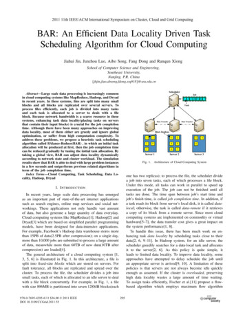
Initial loadLocal costRemote 1s3s2Server(a) Loop 1(b) Loop 2Initial loadLocal costRemote costInitial loadLocal costRemote s2ServerServer(c) Loop 3(d) ResultFig. 6.Finally, we analyse the time complexity of BAR. In thebalance phase, it is shown that BAA is implemented in timeO(max{m n, n log n} · m). In reduce phase, most loopsallocate tasks in time O(m). However, since the last loopneed allocate some tasks to the minimum load servers, it takesO(m log n) time.( There are at most m)loops, so reduce phaseruns in time O m(m 1) m log n) .Combining the running time of the two phases, BAR givestime complexity O(max{m n, n log n} · m).3.33.3t6s1Algorithm 3 Balance-Reduce Algorithm1: procedure BALANCE -R EDUCE(G, Cloc , Crem , Linit )2:define: B, R are total allocations.3:B Balance(G, Cloc , Linit )4:R Reduce(Cloc , Crem , B, Linit )5:return R6: end procedures3Server7.1Combining the balance phase and the reduce phase, thepseudocode of BAlance-Reduce(BAR) is shown in Algorithm3.t7t6s2C. Balance-Reduce Algorithmt54.2t7s13, however, the reduced makespan increase to 7.2 and theexpected makespan is 5.2, so we stop the reduce phase. Finally,we get a total allocation whose makespan is 6.2.Initial loadLocal costRemote costs3An example of the reduce phaseV. P ERFORMANCE E VALUATION3) Calculate the expected makespan of R. The expectedmakespan Mexp equals to the maximum load of serversunder Lp .4) Calculate the remote cost. As task in Lp are data-localand tasks in P are data-remote, the remote task numberRshould be P . Hence, Crem Crem ( P ).5) Allocate tasks. For all tasks tloc / P , we allocate themto Lp (tloc ), so R(tloc ) Lp (tloc ). Then we allocateremote tasks one-by-one. For any task trem P , itis allocated to the server whose load is no more thanRMexp Crem. If there is no appropriate server, weallocate trem to the server with minimum load. Thenwe update the load of the server.6) Return result. If makespanR is larger than the expectedmakespan Mexp , it is impossible to reduce the makespanin the next loops. So a better allocation is selectedbetween R and Rpre , then it is returned.In this section, we present several simulations in order toinvestigate the effectiveness of our algorithm. For comparison,four related task scheduling algorithms are listed as follows: MaxCover-BalAssign(MB)[11]. This algorithm works iteratively to produce a sequence of total allocations, andthen outputs th

data locality, most of them either are greedy and ignore global optimization, or suffer from high computation complexity. . Data Lo-cality, Hadoop, Dryad I. INTRODUCTION In recent years, large scale data processing has emerged as an important part of state-of-the-art internet applications such as search engines, online map services and social .