WIXLIB

34CHEN, KABER, AND DEMPSEYthe number of neurons or the architecture, in general. Nussbaum and Chaffin (1996) developed FNNs for prediction of low-back muscle activation levels and used between threeand eight neurons in a single hidden layer. These numbers were intended to representsmall and large neural architectures. Zurada et al. (1997) also developed multilayer FNNsfor classifying industrial jobs in terms of LBD risk. They used between eight and 20neurons in a hidden layer based on the performance of networks in classifying trainingdata. The number of output neurons in an FNN is determined on the basis of the numberof classes into which a response can be classified. The combination of the number ofhidden neurons and output neurons generates the set of FNNs as part of the first phase ofthe “two-phase” approach mentioned previously.One approach to selecting input variables to a network involves using a multivariateanalysis (MVA) technique (e.g., multiple linear regression (MLR), multiple-discriminateanalysis) to determine the significance of specific inputs and the adequacy of a modelconstructed in them. For example, Killough et al. (1995) used a multivariate analysis ofvariance to identify network input variables having a significant regression relationshipwith a selected network output in advance of defining the architectural characteristics oftheir ANN. The major drawback of using a MVA as a basis for ANN development is thatvery often regression-model prediction accuracy is compromised by violations of assumptions associated with this type of analysis, or there may be insufficient data to accuratelyassess the influence of regressors on the model response and the adequacy of a model, ingeneral. If these methods are not applied correctly in this stage, the prediction accuracy ofthe network may be compromised.Beyond architectural issues, the traditional approach of FNN development, using theEBP algorithm, can suffer from the limitation of “trapping” into poor problem solutions.Unless a good initial overall solution to a problem is provided as a starting point for thisalgorithm, it sometimes traps into a local optimum. For this reason, local search methodssuch as simulated annealing (SA; Marren et al., 1990) have recently been used in conjunction with FNNs to develop better overall data-classification solutions. This methodcan be used to identify a good initial solution to hard combinatorial problems and canescape from a local optimum solution. When combined with a robust and efficient nonlinearprogramming method, such as the conjugate gradient (CG) algorithm, the overall methodcan converge to the optimum solution within the initial region identified through SA (Chenet al., 2000; Masters, 1993).2. THE SINGLE-PHASE BACKWARD-ELIMINATION APPROACHTO FNN DEVELOPMENTTo address the problems in contemporary applications of FNNs to ergonomics, we useda single-phase backward-elimination approach (see Chen et al., 2000) to develop an FNNfor classifying industrial jobs as posing a low or a high risk for LBDs. The main idea ofthis approach is to integrate the work in each phase of the two-phase approach. It directlyrelates the prediction accuracy of the FNN to the development of its architecture, especially the selection of the input variables. Therefore, the FNN generated could be the bestFNN for the classification problem.The single-phase backward-elimination approach is based, in part, on the backwardelimination method of MLR. An FNN with n input variables and m classes of output istrained by using the SA and CG method, and the PCC in validation is recorded. A new

USING FEEDFORWARD NEURAL NETWORKS35FNN is constructed with the same number of input and output neurons, but with h 1hidden neurons. The training and validation for the FNN is continued. If the PCC of thenew FNN is higher than that of the previous FNN, the number of hidden neurons is increased by one to build a new FNN. Subsequently, training and validation is performed.This iterative process is stopped when the PCC of an FNN cannot be improved.The second iteration of the development process considers all the FNNs with n 1input variables. It starts with an FNN with the first variable eliminated from the given setof n variables. With this set of inputs, the same process described earlier is used to findthe FNN with the highest PCC. The process is applied to all possible FNNs with differentsets of n 1 input variables. Comparing the highest PCCs of the FNNs under all of thesedifferent conditions, the best FNN with n 1 input variables is chosen. If its PCC ishigher than the highest PCC found in the previous iteration, the process will be resumedfrom the current best FNN (with the specified n 1 variables) and repeated to find thebest FNN with n 2 input variables. This procedure is terminated if the PCC of the bestFNN found in the current iteration is lower than that found in the previous iteration. Thebest FNN found in the previous iteration is the FNN for the problem.This single-phase approach demonstrated superior results when compared to Zuradaet al.’s (1997) research on the use of the traditional FNN development process for solvingthe same classification problem. Zurada et al. applied the “two-phase” FNN developmentprocedure, presented in Figure 1, to an industrial jobs dataset developed based on a fieldstudy conducted by Marras et al. (1993). The dataset is composed of observations on 235jobs and included a dependent variable, low-back disorder risk, with two discrete levelsof “low” and “high.” The dataset also included five independent variables, describingoccupational risk factors for developing LBDs, including lift rate in number of lifts perhour (LIFTR), peak twist velocity average (PTVAVG), peak moment (PMOMENT), peaksagittal angle (PSUB), and peak lateral velocity maximum (PLVMAX). Zurada et al.used 148 data points from the dataset for training their FNNs; 74 observations on bothlow- and high-risk jobs were selected. The remaining 87 observations were used for validation, including 50 observations on low-risk jobs and 37 observations on high-risk jobs.They found an FNN with all input variables, two output neurons, and 10 hidden neuronsin a single layer to produce the highest percentage of correct job classifications (0.747).The single-phase approach was applied to the Marras et al. (1993) dataset in exactlythe same manner as Zurada et al. (1997) (i.e., the same number of observations on lowand high-risk jobs were used for training and validating networks). Results revealed thehighest PCC for validation (0.793) for a network including four of the five independentvariables represented in the dataset (LIFTR was eliminated) and three hidden neurons inone layer.Not only was the single-phase approach superior in terms of overall classification accuracy but it outperformed Zurada et al.’s (1997) approach in classifying both high- andlow-risk jobs. This is important because there are likely differential costs associated withthe two types of classification errors. Misclassification of high-risk jobs may pose hazards to workers and potential for costly LBDs. Misclassifications of low-risk jobs maypose unnecessary redesign of work systems. Given that resources for ergonomic improvements are often limited or scarce, correctly identifying the risk associated with jobs iscritical. In general, the single-phase approach produced an FNN with better predictionaccuracy and a parsimonious architecture. Most importantly, the match between the desired FNN output and actual risk observations, based on training of the FNN, is moreaccurate when using the SA and CG method, as compared to an EBP algorithm.

36CHEN, KABER, AND DEMPSEY3. SINGLE-PHASE FORWARD-SELECTION APPROACHTO FNN DEVELOPMENTAlthough the results of the single-phase backward-elimination approach to FNN architecting showed improvements over previous work, there are several potential shortcomings to the approach. These shortcomings may be overcome, in part, by forward selectionof input variables in FNN development.The first drawback of the backward-elimination approach is that it requires a largenumber of training samples to develop an FNN. According to Masters (1993), as a rule ofthumb, the minimum number of training samples for an FNN should be twice the numberof connection weights in the FNN. This is because too few training samples may causethe FNN to be overspecified during the training step, affecting its prediction accuracy invalidation. The prediction accuracy of the network may achieve optimality regardless ofwhether the inputs have a causal relationship to outputs. However, performance of thenetwork for a validation dataset may be extremely poor. Therefore, suppose there is aproblem with 20 independent variables and one dependent variable with two classes. Ifthe backward-elimination approach is used, the starting structure of a single-hidden-layerFNN for the problem is composed of 20 input nodes, two output nodes, and six hiddennodes [Int (20 2)1/2 6]. Note that a bias node is added to both the input and hiddenlayers, and the number of connection weights can be calculated using the equation: n 1! h h 1! m, where n is the number of input nodes, h is the number ofhidden nodes, m is the number of output nodes, and the “1” refers to the bias nodes.Therefore, the number of weights of the FNN is equal to (20 1) 6 (6 1) 2 140, and the minimum number of training samples for the FNN, according to Masters’(1993) rule, is 280. Of course, this number increases as the number of hidden nodes increases. Suppose also that the final FNN generated by using the backward-eliminationapproach includes 10 input variables and four hidden nodes. The number of weights ofthe FNN is equal to: (10 1) 4 (4 1) 2 54, so the required minimum numberof training samples is equal to 108.For the same problem, if the forward-selection idea of MLR is applied to the FNNdevelopment, the starting structure of the FNN is composed of one input variable andtwo hidden nodes. The number of weights of the FNN is equal to (1 1) 2 (2 1) 2 10, and the minimum number of training samples for the FNN is 20. Implementingthe forward-selection idea, one variable will be added to the FNN at a time. Assumingthat the forward-selection procedure will generate the same final FNN as that generatedby using the backward-elimination approach, the minimum number of training samplesrequired for applying this procedure should not exceed 108. Making comparison with thenumber of samples required for the backward-elimination approach, there is an enormoussaving in terms of the data collection required to achieve the solution to the problem. Thisbenefit could prove especially important for existing datasets with a high percentage ofmissing observations. For example, one of us (C.-L. C.) previously addressed a problemwith 18 independent variables, one dependent variable, and a dataset containing 168training samples. Unfortunately, approximately 19% of the intended observations oneach variable (specific settings and responses) were missing across training samples(Observations on each variable were not necessarily missing for the same training samples.)When all samples with missing data were eliminated, only 41 complete samples remained. This number was far less than the minimum number of samples recommended byMasters (1983), which is equal to: 2 (18 1) 6 (6 1) 2 256, and would be

USING FEEDFORWARD NEURAL NETWORKS37required to use the backward-elimination approach. Subsequently, the training sampleswere examined by considering one independent variable, two independent variables, threeindependent variables, and four independent variables at a time. It was found that theaverage number of complete samples (no missing data) for four independent variableswas 80. Comparing this number with Masters’ minimum number of training samples forFNN development with four input variables, [2 (4 1) 3 (3 1) 2] 46,revealed that the forward-selection approach could be a viable way of solving the problem.With respect to the effect of missing data on FNN development, if a backwardelimination procedure is applied for input selection, during the first few iterations of theprocess the number of data points available may be small in comparison to the number ofinputs, and network performance will be compromised. Accordingly, the input variableselection and final result (i.e., identification of the best FNN generated) will be influenced by the missing data. If a forward-selection procedure is applied, since input variables are added to the FNN one by one, a relatively large number of data points may existfor training and validation in comparison to the number of inputs at least for the first fewiterations of the process. The decisions made in these iterations will be more accurate,and the missing data will have less of an influence on the final result.Asecond major shortcoming of the backward-elimination approach is that it requires substantial computation time. This is especially critical for problems with a large number ofindependent variables. In addressing the aforementioned 18-variable problem, the missingdata were replaced with a value of “0,” and a FNN was trained with the 18 input variablesand six hidden nodes in a single hidden layer. Training the FNN required 665 central processing unit (CPU) seconds on an 833-MHz personal computer (PC). Using the same dataset, 18 different FNNs were trained with a single input node and two hidden nodes. EachFNN used one of the 18 independent variables included in the problem dataset as an inputvariable. Each FNN required less than 4 s to train on the same PC. In general, the backwardelimination approach starts by defining an FNN with 18 input nodes, then 17 FNNs with17 input nodes are generated, followed by the development of 16 FNNs with 16 inputnodes, and so on. This procedure continues until a stopping criterion is satisfied. Conversely, the forward-selection approach starts by defining 18 FNNs with one input node,then 17 FNNs with two input nodes, followed by 16 FNNs with three input nodes, and soon, until a stopping criterion is satisfied. As described, the training time for an FNN witha relatively large architecture is considerably longer than that of an FNN with a smallstructure. With this in mind, achieving an overall solution to the problem using the forwardselection approach may be far more efficient than the backward-elimination approach.A third and final shortcoming of the backward-elimination approach is that it does notprovide clear insight into the utility of each independent variable for classifying networkoutput. This is because the backward-elimination procedure removes input variables froma network in order of insignificance. It does not investigate the classification effect ofindividual input variables on the output variable. This problem can be addressed by theforward-selection approach because it begins by analyzing the training data for an FNNwith one input variable and subsequently includes inputs in the network in order of significance for explaining outputs.Considering the problems with a backward-elimination based approach and the potential benefits of using a forward-selection-based approach, we applied a new procedure tothe classification problem initially explored by Zurada et al. (1997), and to which we previously applied the single-phase backward-elimination approach to network development(Chen et al., 2000). Our expectation was that the performance of the resulting FNN would

38CHEN, KABER, AND DEMPSEYbe at least comparable to the best network generated based on the backward-eliminationbased approach for complete datasets and that the forward-selection method would provide superior results with datasets missing observations.3.1. Procedure for the Forward-Selection ApproachThe procedure for the forward-selection approach is largely an adaptation of the Chenet al. (2000) method. It represents an incremental advance in the FNN development procedure. A detailed flow diagram of the procedure is presented in Figure 2.The first five steps of the procedure are similar to those presented by Chen et al. (2000).They involve specifying the variables of the problem, collecting data on them, and creating training and validation datasets to use in the network development.Initially, an FNN is constructed with one input neuron n 1) and two output neurons m 2) (Step 6). The number of hidden neurons in the network is specified using Masters’ (1993) equation (i.e., h Int [ m n! 1/2 ], and h ⱖ 2). This FNN is trained using theSA and CG algorithm (Step 7). The prediction capability of the FNN is determined usinga validation dataset and recorded (Step 8). A new FNN is then constructed with the samenumber of input and output neurons, but with h 1 hidden neurons. The training andvalidation of this FNN is conducted. If the prediction performance of the new FNN isgreater than that of the FNN with h hidden neurons, then another FNN is constructed withh 2 hidden neurons. Subsequently, the training and validation for this new network isconducted, and the prediction performance is compared with that of the FNN includingh 1 hidden neurons. This iterative process continues until the performance of the FNNdoes not improve (Steps 7–9).Subsequently, a new set of FNNs is constructed using a different input variable fromthe dataset. The same process involving manipulation of the number of hidden neurons inthe FNN, including the new input variable, is conducted. The performance of the FNNsdeveloped on the basis of the various input variables is compared, and the input resultingin the best performing FNN is selected for inclusion in the set for the final NN solution(Steps 5 and 10–12).The second iteration of this procedure involves considering all the FNNs with two inputvariables. It starts with an FNN, including the input variable selected based on the resultsof the first iteration, and a new input variable added from the given set of n variables(Steps 15–18). With these inputs, the process described previously is used to find the FNNwith the highest PCC. All possible FNNs with different sets of two input variables are considered. The FNNs with the highest PCCs for these conditions are then compared, and theinput variables for the best FNN are chosen for the final NN solution (Steps 19–24). If theFNN PCC for the second iteration is found to be higher than the PCC for the best FNN produced through the first iteration, then the process is continued from the current best FNN(with the two established input variables) to find the best FNN with three input variables.The procedure is terminated if the PCC of the best FNN found in the current iteration islower than that found in the previous iteration (Step 25). The best FNN found in theprevious iteration is the final NN solution to the classification problem (Step 26).4.COMPUTATIONAL RESULTSThe dataset developed by Marras et al. (1993), and evaluated by Zurada et al. (1997) andChen et al. (2000), was used to assess the performance of the forward-selection approach.To observe results of the new approach under a condition where a high percentage of data

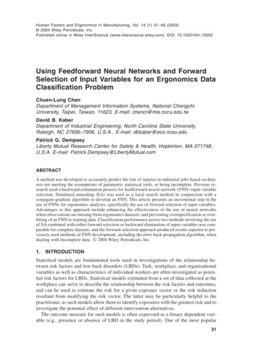
39USING FEEDFORWARD NEURAL NETWORKSTABLE 1.Classification Results for Three Methods Using Reduced Training DatasetsConfusion MatrixLogistic 1560.586MDA multiple discriminant analysis; FNN feedforward neural network.is missing, we decimated the Marras et al. dataset. First, we selected 100 of the 148 training samples used by Zurada et al. and Chen et al. Specifically, we used the first 50 samples from each of the training datasets on low- and high-risk jobs (which included 74observations in the analysis by Zurada et al.). The remainder of samples were retained forvalidation of the network. Subsequently, we reduced the number of data points on eachvariable included in the overall dataset by 20%. We devised a simple test of each datapoint to determine if it should be deleted. The test compared a prespecified thresholdvalue with a randomly generated value (0.20) between 0 and 1. If the random value wasless than the threshold value, the data point was deleted. In general, we included far fewersamples in the FNN training datasets than were used in Chen et al., and we decimated thedata such that the overall number of observations for training was less than would berecommended for developing an FNN using historical methods.The purpose of this data handling was to generate a dataset for which the backwardelimination approach and other commonly used analytical tools would not be expected toperform well. Once we deleted data points from the reduced training and validation subsets, it was found that there were only 25 complete samples remaining for training, and29 samples in the validation dataset. The minimum number of samples for training anFNN with five input variables is: [(5 1) 3 (3 1) 2] 2 52. It is important tonote that this would be the minimum number of samples required when using the backwardelimination approach to generate an FNN solution for this ergonomics classification problem by beginning with all five input variables.As points of comparison for t

University, Taipei, Taiwan, 11623, E-mail: chencl@mis.nccu.edu.tw David B. Kaber Department of Industrial Engineering, North Carolina State University, Raleigh, NC 27695-7906, U.S.A., E-mail: dbkaber@eos.ncsu.edu . pendent variables and its response can be classified into two classes, Masters would rec-ommend constructing an initial FNN .