WIXLIB

x 1 , x 1 x 2 , x 1 . .······. x 1 , x n x 2 , x n . . x n , x 1 ··· x n , x n ABC DMarkov Transition FieldWe propose a framework similar to (Campanharo et al.2011) for encoding dynamical transition statistics, but weextend that idea by representing the Markov transition probabilities sequentially to preserve information in the time domain.Given a time series X, we identify its Q quantile bins andassign each xi to the corresponding bins qj (j [1, Q]).Thus we construct a Q Q weighted adjacency matrix Wby counting transitions among quantile bins in the manner ofa first-order Markov chain along the time axis. wi,j is givenby the frequency with which a point in the quantile qj is followed by a point in the quantile qi . After normalization byPj wij 1, W is the Markov transition matrix. It is insensitive to the distribution of X and temporal dependency ontime steps ti . However, getting rid of the temporal dependency results in too much information loss in matrix W . Toovercome this drawback, we define the Markov TransitionField (MTF) as follows: w ··· wij x1 qi ,x1 qjij x1 qi ,xn qj···.···wij x2 qi ,xn qj . .wij xn qi ,xn qjB0.0830.5830.2600.083C00.3340.5220.167DMarkov Transition Matrx000.2180.75DDThe GAF has several advantages. First, it provides a wayto preserve the temporal dependency, since time increases asthe position moves from top-left to bottom-right. The GAFcontains temporal correlations because G(i,j i j k) represents the relative correlation by superposition of directionswith respect to time interval k. The main diagonal Gi,i isthe special case when k 0, which contains the originalvalue/angular information. With the main diagonal, we willapproximately reconstruct the time series from the high levelfeatures learned by the deep neural network. However, theGAF is large because the size of Gramian matrix is n nwhen the length of the raw time series is n. To reduce thesize of the GAF, we apply Piecewise Aggregation Approximation (Keogh and Pazzani 2000) to smooth the time seriesand while keeping trends. The full procedure for generatingthe GAF is illustrated in Figure 1. wij x2 qi ,x1 qjM . .wij xn qi ,x1 qjTypical Time Series(5)A0.9170.08300(6)We build a Q Q Markov transition matrix (say, W )by dividing the data (magnitude) into Q quantile bins. Thequantile bins that contain the data at time stamp i and j (temporal axis) are qi and qj (q [1, Q]). Mij in MTF denotesthe transition probability of qi qj . That is, we spreadout matrix W which contains the transition probability onthe magnitude axis into the MTF matrix by considering thetemporal positions.By assigning the probability from the quantile at time stepi to the quantile at time step j at each pixel Mij , the MTFM actually encodes the multi-span transition probabilitiesCCBBAAMarkov Transition FieldBlurred Markov Transition FieldFigure 2: Illustration of the proposed encoding map ofMarkov Transition Field. X is a sequence of typical timeseries in dataset ’ECG’. X is firstly discretized into Q quantile bins. Then we calculate its Markov Transition Matrix Wand finally build its MTF with eq. (6). In addition, we reduce the image size from 96 96 to 48 48 by averagingthe pixels in each non-overlapping 2 2 patch.of the time series. Mi,j i j k denotes the transition probability between the points with time interval k. For example, Mij j i 1 illustrates the transition process along thetime axis with a skip step. The main diagonal Mii , whichis a special case when k 0 captures the probability fromeach quantile to itself (the self-transition probability) at timestep i. To make the image size manageable and computationmore efficient, we reduce the MTF size by averaging the pixels in each non-overlapping m m patch with the blurringkernel { m12 }m m . That is, we aggregate the transition probabilities in each subsequence of length m together. Figure 2shows the procedure to encode time series to MTF.Tiled Convolutional Neural NetworksTiled Convolutional Neural Networks (Ngiam et al. 2010)are a variation of Convolutional Neural Networks that usetiles and multiple feature maps to learn invariant features.Tiles are parameterized by a tile size k to control the distance over which weights are shared. By producing multiple feature maps, Tiled CNNs learn overcomplete representations through unsupervised pretraining with TopographicICA (TICA).A typical TICA network is actually a double-stage optimization procedure with squares and square root nonlinearities in each stage, respectively. In the first stage, theweight matrix W is learned while the matrix V is hardcoded to represent the topographic structure of units. Moreprecisely, given a sequence of inputs {xh }, the activationin the second stage is fi (x(h) ; W, V ) qPof each unitPq(h) 2pk 1 Vik (j 1 Wkj xj ) . TICA learns the weight matrix W in the second stage by solving the following:minimizeWpn XXh 1 i 1Tsubject to W Wfi (x(h) ; W, V ) I(7)

Convolutional IFeature maps 𝑙 6Receptive Field 8 8Convolutional II TICA Pooling IITICA Pooling I.Linear SVMTable 1: Tiled CNN error rate on training set and test set.DATASET.Untied weights 𝑘 2.Pooling Size 3 3.Pooling Size 3 3Receptive Field 3 3Figure 3: Structure of the tiled convolutional neural network.We fix the size of receptive field to 8 8 in the first convolutional layer and 3 3 in the second convolutional layer.Each TICA pooling layer pools over a block of 3 3 inputunits in the previous layer without wraparound the boardersto optimize for sparsity of the pooling units. The number ofpooling units in each map is exactly the same as the numberof input units. The last layer is a linear SVM for classification. We construct this network by stacking two Tiled CNNs,each with 6 maps (l 6) and tiling size k 2.Above, W Rp q and V Rp p where p is the numberof hidden units in a layer and q is the size of the input. V isa logical matrix (Vij 1 or 0) that encodes the topographicstructure of the hidden units by a contiguous 3 3 block.The orthogonality constraint W W T I provides diversityamong learned features.Neither GAF nor MTF images are natural images; theyhave no natural concepts such as “edges” and “angles”.Thus, we propose to exploit the benefits of unsupervised pretraining with TICA to learn many diverse features with localorthogonality. In addition, Ngiam et al. empirically demonstrate that tiled CNNs perform well with limited labeled databecause the partial weight tying requires fewer parametersand reduces the need for a large amount of labeled data. Ourdata from the UCR Time Series Repository (Keogh et al.2011) tends to have few instances (e.g., the “yoga” datasethas 300 labeled instance in the training set and 3000 unlabeled instance in the test set), tiled CNNs are suitable for ourlearning task.Typically, tiled CNNs are trained with two hyperparameters, the tiling size k and the number of feature maps l.In our experiments, we directly fixed the network structureswithout tuning these hyperparameters in loops for severalreasons. First, our goal is to explore the expressive power ofthe high level features learned from GAF and MTF images.We have already achieved competitive results with the default deep network structures that Ngiam et al. used for image classification on the NORB image classification benchmark. Although tuning the parameters will surely enhanceperformance, doing so may cloud our understanding of thepower of the representation. Another consideration is computational efficiency. All of the experiments on the 12 “hard”datasets could be done in one day on a laptop with an Intel i7-3630QM CPU and 8GB of memory (our .3610.4110.30.4830.1760.243platform). Thus, the results in this paper are a preliminarylower bound on the potential best performance. Thoroughlyexploring the deep network structures and parameters willbe addressed in future work. The structure and parametersof the tiled CNN used in this paper are illustrated in Figure3.Classifying Time Series Using GAF/MTFWe apply Tiled CNNs to classify using GAF and MTF representation on twelve tough datasets, on which the classification error rate is above 0.1 with the state-of-the-art SAXBoP approach (Lin, Khade, and Li 2012; Oates et al. 2012).More detailed statistics are summarized in Table 2. Thedatasets are pre-split into training and testing sets for experimental comparisons. For each dataset, the table gives itsname, the number of classes, the number of training and testinstances, and the length of the individual time series.Experimental SettingIn our experiments, the size of the GAF image is regulatedby the the number of PAA bins SGAF . Given a time series X of size n, we divide the time series into SGAF adjacent, non-overlapping windows along the time axis andextract the means of each bin. This enables us to constructthe smaller GAF matrix GSGAF SGAF . MTF requires thetime series to be discretized into Q quantile bins to calculatethe Q Q Markov transition matrix, from which we construct the raw MTF image Mn n afterwards. Before classification, we shrink the MTF image size to SM T F SM T Fby the blurring kernel { m12 }m m where m d SMnT F e. TheTiled CNN is trained with image size {SGAF , SM T F } {16, 24, 32, 40, 48} and quantile size Q {8, 16, 32, 64}.At the last layer of the Tiled CNN, we use a linear soft margin SVM (Fan et al. 2008) and select C by 5-fold cross validation over {10 4 , 10 3 , . . . , 104 } on the training set.For each input of image size SGAF or SM T F and quantile size Q, we pretrain the Tiled CNN with the full unlabeled dataset (both training and test set) to learn the initialweights W through TICA. Then we train the SVM at the lastlayer by selecting the penalty factor C with cross validation.

Table 2: Summary statistics of standard dataset and comparative 70.4460.0930.16Finally, we classify the test set using the optimal hyperparameters {S, Q, C} with the lowest error rate on the trainingset. If two or more models tie, we prefer the larger S and Qbecause larger S helps preserve more information throughthe PAA procedure and larger Q encodes the dynamic transition statistics with more detail. Our model selection approach provides generalization without being overly expensive computationally.Results and DiscussionWe use Tiled CNNs to classify GAF and MTF representations separately on the 12 datasets. The training and test error rates are shown in Table 1. Generally, our approach isnot prone to overfitting as seen by the relatively small difference between training and test set errors. One exception isthe Olive Oil dataset with the MTF approach where the testerror is significantly higher.In addition to the risk of potential overfitting, MTF hasgenerally higher error rates than GAF. This is most likely because of uncertainty in the inverse image of MTF. Note thatthe encoding function from time series to GAF and MTF areboth surjective. The map functions of GAF and MTF willeach produce only one image with fixed S and Q for eachgiven time series X . Because they are both surjective mapping functions, the inverse image of both mapping functionsis not fixed. As shown in a later section, we can approximately reconstruct the raw time series from GAF, but it isvery hard to even roughly recover the signal from MTF. GAFhas smaller uncertainty in the inverse image of its mappingfunction because such randomness only comes from the ambiguity of cos(φ) when φ [0, 2π]. MTF, on the other hand,has a much larger inverse image space, which results in largevariation when we try to recover the signal. Although MTFencodes the transition dynamics which are important features of time series, such features seem not to be sufficientfor recognition/classification tasks.Note that at each pixel, Gij , denotes the superstition ofthe directions at ti and tj , Mij is the transition probabilityfrom quantile at ti to quantile at tj . GAF encodes static information while MTF depicts information about dynamics.From this point of view, we consider them as two “orthogo-nal” channels, like different colors in the RGB image space.Thus, we can combine GAF and MTF images of the samesize (i.e. SGAF SM T F ) to construct a double-channel image (GAF-MTF). Since GAF-MTF combines both the staticand dynamic statistics embedded in raw time series, we positthat it will be able to enhance classification performance. Inthe next experiment, we pretrain and train the Tiled CNNon the compound GAF-MTF images. Then, we report theclassification error rate on test sets.Table 2 compares the classification error rate of our approach with previously published performance results offive competing methods: two state-of-the-art 1NN classifiersbased on Euclidean distance and DTW, the recently proposed Fast-Shapelets based classifier (Rakthanmanon andKeogh 2013), the classifier based on Bag-of-Patterns (BoP)(Lin, Khade, and Li 2012; Oates et al. 2012) and the most recent SAX-VSM approach (Senin and Malinchik 2013). Ourapproach outperforms 1NN-Euclidean, fast-shapelets, andBoP, and is competitive with 1NN-DTW and SAX-VSM.In addition, by comparing the results between Table 2 andTable 1, we verified our assumption that combined GAFMTF images have better expressive power than GAF orMTF alone for classification. GAF-MTF achieves the lowertest error rate on ten datasets out of twelve (except for thedataset Adiac and Beef). On the Olive Oil dataset, the training error rate is 6.67% and the test error rate is 16.67%. Thisdemonstrates that the integration of both types of imagesinto one compound image decreases the risk of overfittingas well as enhancing the overall classification accuracy.Analysis on Features and Weights Learnedthrough Tiled CNNsIn contrast to the cases in which the CNN is applied in natural image recognition tasks, neither GAF nor MTF has natural interpretations of visual concepts like “edges” or “angles”. In this section we analyze the features and weightslearned through Tiled CNNs to explain why our approachworks.As mentioned earlier, the mapping function from time series to GAF is surjective and the uncertainty in its inverseimage comes from the ambiguity of the cos(φ) when φ

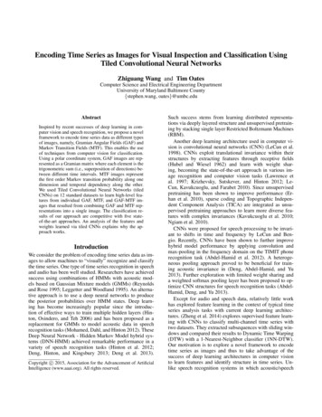
Figure 4: (a) Original GAF and its six learned feature mapsbefore the SVM layer in Tiled CNN (top left), and (b) rawtime series and approximate reconstructions based on themain diagonal of six feature maps (top right) on ’50Words’dataset; (c) Original MTF and its six learned feature mapsbefore the SVM layer in Tiled CNN (bottom left), and (d)curve of self-transition probability along time axis (maindiagonal of MTF) and approximate reconstructions basedon the main diagonal of six feature maps (bottom right) on”SwedishLeaf” dataset.[0, 2π]. The main diagonal of GAF, i.e. {Gii } {cos(2φi )}allows us to approximately reconstruct the original time series, ignoring the signs byrcos(2φ) 1cos(φ) (8)2MTF has much larger uncertainty in its inverse image,making it hard to reconstruct the raw data from MTF alone.However, the diagonal {Mij i j k } represents the transition probability among the quantiles in temporal order considering the time interval k. We construct the self-transitionprobability along the time axis from the main diagonal ofMTF like we do for GAF. Although such reconstructionsless accurately capture the morphology of the raw time series, they provide another perspective of how Tiled CNNscapture the transition dynamics embedded in MTF.Figure 4 illustrates the reconstruction results from six feature maps learned before the last SVM layer on GAF andMTF. The Tiled CNN extracts the color patch, which is essentially a moving average that enhances several receptivefields within the nonlinear units by different trained weights.It is not a simple moving average but the synthetic integration by considering the 2D temporal dependencies amongdifferent time intervals, which is a benefit from the Gramianmatrix structure that helps preserve the temporal information. By observing the rough orthogonal reconstruction fromeach layer of the feature maps, we can clearly observe thatthe tiled CNN can extract the multi-frequency dependencies through the convolution and pooling architecture on theGAF and MTF images to preserve the trend while addressing more details in different subphases. As shown in Figure4(b) and 4(d), the high-leveled feature maps learned by theTiled CNN are equivalent to a multi-frequency approximatorof the original curve.Figure 5: learned sparse weights W for the last SVM layerin Tiled CNN (left) and its orthogonality constraint byW W T I (right).Figure 5 demonstrates the learned sparse weight matrixW with the constraint W W T I, which makes effectiveuse of local orthogonality. The TICA pretraining providesthe built-in advantage that the function w.r.t the parameterspace is not likely to be ill-conditioned as W W T 1. Asshown in Figure 5 (right), the weight matrix W is quasiorthogonal and approaching 0 without very large magnitude.This implies that the condition number of W approaches 1helps the system to be well-conditioned.Conclusions and Future WorkWe created a pipeline for converting time series data intonovel representations, GAF and MTF images, and extractedhigh-level features from these using Tiled CNN. The features were subsequently used for classification. We demonstrated that our approach yields competitive results whencompared to state-of-the-art methods when searching a relatively small parameter space. We found that GAF-MTFmulti-channel images are scalable to larger numbers ofquasi-orthogonal features that yield more comprehensiveimages. Our analysis of high-level features learned fromTiled CNN suggested that Tiled CNN works like a multifrequency moving average that benefits from the 2D temporal dependency that is preserved by Gramian matrix.Important future work will involve applying our methodto massive amounts of data and searching in a more complete parameter space to solve the real world problems. Weare also quite interested in how different deep learning architectures perform on the GAF and MTF images. Anotherinteresting future work is to model time series through GAFand MTF images. We aim to apply learned time series models in regression/imputation and anomaly detection tasks. Toextend our methods to the streaming data, we suppose todesign the online learning approach with recurrent networkstructures.

ReferencesAbdel-Hamid, O.; Mohamed, A.-r.; Jiang, H.; and Penn, G. 2012.Applying convolutional neural networks concepts to hybrid nnhmm model for speech recognition. In Acoustics, Speech and Signal Processing (ICASSP), 2012 IEEE International Conference on,4277–4280. IEEE.Abdel-Hamid, O.; Deng, L.; and Yu, D. 2013. Exploring convolutional neural network structures and optimization techniques forspeech recognition. In INTERSPEECH, 3366–3370.Campanharo, A. S.; Sirer, M. I.; Malmgren, R. D.; Ramos, F. M.;and Amaral, L. A. N. 2011. Duality between time series and networks. PloS one 6(8):e23378.Deng, L.; Abdel-Hamid, O.; and Yu, D. 2013. A deep convolutional neural network using heterogeneous pooling for tradingacoustic invariance with phonetic confusion. In Acoustics, Speechand Signal Proces

novel way to understand time series. As time increases, cor-responding values warp among different angular points on the spanning circles, like water rippling. The encoding map of equation 2 has two important properties. First, it is bijec-tive as cos( ) is monotonic when 2[0;ˇ]. Given a time