Transcription
CS2291From Classical To Hip-Hop: Can Machines LearnGenres?Aaron Kravitz, Eliza Lupone, Ryan DiazAbstract—The ability to classify the genre of a song is aneasy task for the human ear. After listening to a song for justseveral seconds, it is often not difficult to take note of that song’scharacteristics and subsequently identify this genre. However,this task is one that computers have historically not been ableto solve well, at least not until the advent of more sophisticatedmachine learning techniques. Our team explored several of thesetechniques over the course of this project and successfully builta system that achieves 61.873% accuracy in classifying musicgenres. This paper discusses the methods we used for exploratorydata analysis, feature selection, hyperparameter optimization,and eventual implementation of several algorithms for classification.I. I NTRODUCTIONHISTORICALLY, attempts made by others to build musicgenre classification systems have yielded fine but notextraordinary results. Some who used the same dataset thatwe used for our project, which comprises one million songseach belonging to one of ten different genres, often chose toreduce the number of genres they attempted to identify, whilethose who decided to work with all ten genres only achievedaccuracy of 40% [1].The hardest part of music classification is working with timeseries data. The cutting edge of machine learning research islooking into more effective ways of extracting features fromtime series data, but is still a long way off. The most promisingattempt is done by Goroshin et. al in their paper UnsupervisedFeature Learning from Temporal Data [2].The problem with temporal data is that the number offeatures varies per each training example. This makes learninghard, and in particular makes it hard to extract information onexactly what the algorithm is using to “learn”. Algorithmsthat extract temporal features can be thought of as extractinga more reasonably sized set of features that can be learnedfrom. To address the difficulties of working with temporaldata, we used the idea of an acoustic fingerprint [3] to extract aconstant sized number of features from each song, improvingour accuracy on the testing set substantially.We also used Bayesian Optimization, a relatively moderntechnique, to optimize the hyperparameters of our classification algorithms. This increased our accuracy by a fewpercentage points, and is substantially faster than grid searchand leads to better results than random guessing.In short, the task of developing a music genre classificationalgorithm is not a trivial one, and often requires substantialtuning. The best models we discuss in this paper achieve anaccuracy of 61.9%.II. T HE DATASET AND F EATURESFor this project we used the Million Song Genre Dataset,made available by LabROSA at Columbia University [4].This dataset consists of one million popular songs andrelated metadata and audio analysis features such as songduration, tempo, time signature, timbre for each “segment”,and key. In this dataset, each training example is a trackcorresponding one song, one release, and one artist. Amongthe many features that this dataset contains for each track isgenre, which was of obvious importance to our project as it isthe “ground truth” which we aimed to predict with our models.In particular, there are 10 genre lables, distributed according toTable I. This dataset is clearly imbalanced, making the abilityto accurately classify genres other than ”classic pop and rock”,which makes up about 40% of the dataset, a challenge.We changed the original dataset so as to not increase thesize of the features to over 100, while adding to the abilityto differentiate between genres. The original Million SongDataset contains timbre vectors for each segment of each song,where a segment is defined as a small section of the song,usually denoting when a new note comes in. The creators ofthe dataset performed MFCC on the data, which is explained ingreater detail in Sahidullah and Saha [5], and then performedPCA on the results of MFCC to separate the timbre of eachsegment into 12 principle components. The genre dataset onlyincludes the average and variance of each of these segments,which we felt did not contain enough information to describethe data. To remedy this issue, the solution we came up withwas to take the most meaningful segment of the song, usinga variation on the idea of an acoustic fingerprint [3].To achieve this, we used a variation on the idea of anacoustic fingerprint [6]. Research shows that when a person islistening to a piece of music, the brain’s attention is heightenedduring transitions, which frequently coincide with the loudestparts of the music. As such, we decided determine the loudestpoint of each song in our dataset and use the correspondingtimbre feature vector for that segment, an idea that is basedupon work done by Vinod Menon at the Stanford School ofMedicine [7]. The use of this feature improved our modelaccuracy to approximately 58% from around 55% originally.For further improvements, we multiplied the loudness of thatparticular segment and the individual timbres of that segment,which boosted accuracy to 60%.To get a better understanding of the dataset, we first normalized and scaled the dataset, and then plotted the data usingPCA in Fig. 2. We then plotted the data with the new addedfeatures, which does seem to have slightly better clustering of
CS2292classes in Fig. 3.III. M ETHODSFig. 1: Random Forest Learning Curveimprovement upon simple bootstrap aggregation of trees as itdecorrelates the trees [8]. For the purposes of our project, weused python’s sklearn package to construct a random forest onour test data set. We first used Bayesian optimization, whichis explained in greater detail in section 5, to tune severalhyperparameters. The results of this optimization indicated thatthe optimal minimum number of samples required to split aninternal node in a tree is 2, the optimal minimum number ofsamples that must be in a newly created leaf is 1, and theoptimal number of trees in the forest is 300. Having tunedthese parameters, we built a random forest classifier using ourtraining set, which we then used to make genre predictionsfor our test set. For each split we considered p n features.The random forest achieved accuracy of 61.9% and an F1score of 57.9%. The learning curve for this method is shownin Fig. 1, and while our results seem to be an improvementupon those of previous years, the random forest suffers fromhigh variance. That is to say, the model captures too much ofthe variance and noise in the training set, and as a result thegeneralization error suffers.TABLE I: MSD Genre Dataset StatsticsA. Random ForestAfter completing preliminary exploratory data analysis, weshifted our focus to various supervised learning methods,turning first to tree-based methods, which segment the featurespace of a data set into distinct, non-overlapping regionsusing a greedy approach known as recursive binary splitting.Prediction of a test example using a classification tree isperformed by determining the region to which that examplebelongs, and then taking the mode of the training observationsin that region. A classification tree is “grown” by successivelysplitting the predictor space at a single cutpoint which leadsto the greatest possible reduction in some chosen measure.For our project, we chose as our measure the Gini index (G),which is often thought of as a measure of region purity:G KXGenreclassic pop and rockclassicaldance and electronicafolkhip-hopjazz and bluespopmetalpunksoul and reggaeTotal:Counts23, 8951, 8744, 93513, 1924344, 3342, 1031, 6173, 2004, 01659, 3%5.37%6.74%100%p̂mk (1 p̂mk )k 1where K is the number of classes and p̂mk is the proportionof training observations belonging to the kth class in the mthregion. Thus, for every iteration of recursive binary splitting,the splitpoint s is chosen so as to minimize the Gini index andthus maximize the purity of each of the regions. This splittingof the feature space continues until a stopping criterion isreached (for example, if each region in the feature spacecontains fewer than a certain number of training observations).While one single classification tree might not have extraordinary predictive accuracy in comparison to other machinelearning methods, aggregation of decision trees can substantially improve performance. For our project, we chose to usea random forest of classification trees as one of our predictionmethods. Random forests are constructed by building a numberof decision trees on bootstrapped observations, where eachsplit in each tree is decided by examining a random sample ofp out of n features; in this way the random forest method is anFig. 2: PCA With Original FeaturesB. Gaussian Discriminant AnalysisIn addition to tree-based methods, we also explored twodifferent types of Gaussian discriminant analysis. First, weperformed linear discriminant analysis on our training setusing interactive polynomial features of degree 2. Beforerunning the analysis, we created the interactive features bycomputing the (element-wise) product of every pair of distinct
CS2293Fig. 3: PCA With Added FeaturesFig. 4: Linear Discriminant Analysis Learning Curvefeatures. That is to say, for every pair of features n1 , n2where n1 6 n2 , we added n1 n2 to our feature space.After completing this pre-processing, we used python’s sklearnpackage to perform linear discriminant analysis. This methodassumes that our observations x1 , x2 , . . . xn are drawn froma multivariate Gaussian distribution with class-specific meanvectors and a common covariance matrix. Thus, the classifierassumes that an observation from the jth class, for example,is drawn from a distribution N (µj , Σ). The assumption thateach class has the same covariance matrix Σ forces thedecision boundaries in the feature space generated by lineardiscriminant analysis to be linear. The diagnostic results ofthis analysis are summarized in Table II.1) Gaussian Processes: As the prior to our Bayesian optimization problem, we used a Gaussian Process (GP). GaussianProcesses are defined by a multivariate Gaussian distributionover a finite set of points [9]. As more points are observed,the prior is updated, as in 5. What makes Gaussian processesuseful for Bayesian optimization is that we can compute themarginal and conditional distributions in closed form. Formore information on Gaussian Processes, consult Rasmussenand Williams [10].TABLE II: LDA DiagnosticsGenreClassic pop and rockPunkFolkPopDance and electronicaMetalJazz and bluesClassicalHip-hopSoul and reggaeAverage / 1920Fig. 5: Gaussian Process PriorC. Bayesian OptimizationBayesian optimization tries to address the global optimization problemx arg max f (x)x Xwhere f(x) is a black box function, meaning that we haveknowledge of the input and output of the function, but haveno idea how the function works. Bayesian optimization is away of solving this optimization problem effectively.To use Bayesian optimization, we first decide on a priordistribution for the unknown functions. This essentially captures our belief about the family of functions that the unknownfunction comes from. The then decide on an acquisitionfunction, which is used to select the next point to test [9].2) Acquisition Function: In order to optimize our function,we want to test points that have the highest chance of being anargmax. Our function f (x) is drawn from a Gaussian processprior, meaning yn N (f (xn ), ν). The acquisition function isthe function the chooses the next point to try. With a Gaussianprocess, there are a few acquisition functions to choose from,but the one we used was expected improvement.Expected improvement chooses the point that maximizes theexpected improvement over our current best point [11]. Witha Gaussian process, this has a closed forma(x X1:t ) E (max{0, ft 1 (x) ft (x )} X1:t ) σ ( uΦ( u) φ(u))
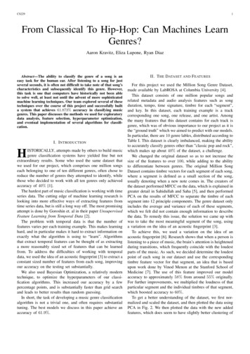
CS2294ClassifierBernoulli Naive BayesMultinomial Naive BayesLatent Dirichlet Allocation (10 topics)Latent Dirichlet Allocation (100 0.54F10.540.500.410.41TABLE III: Results on 10500 training size, 4500 test sizes.t u ymax µσWe will not go into the details of the closed form here, butsee Snoek et al. for details [9].3) Bayesian Optimization of Algorithms: We used Bayesianoptimization to tune the Random Forests algorithm and theSVMs. SVMs did not perform very well on the data originally,but after tuning the hyperparameters, the F1-score increasedfrom around .45 to .51. This is a non-negligible increasethat required performing only 25 iterations of Bayesian optimization in a couple of hours, as opposed to the hundredsof iterations required by grid search, which did not evenfinish running on the dataset provided after 12 hours. Forrandom forests, the accuracy of the classifier increased from59.1% to 61.9% using Bayesian optimization. This is anincrease of about 3% percent, with minimal work from theimplementation side. Bayesian optimization took about anhour to find a reasonable optimum, while grid search again didnot complete in a reasonable amount of time. The paramaterspace examined by each of these algorithms contained 60, 000different configurations of hyperparameters, so the fact thatBayesian optimization was significantly more efficient is nota surprise.D. Lyrical ModelingThe Million Song Dataset supplied a subset of data of210, 519 songs with lyrics in a bag-of-word (term frequencycounts) format. From this data set we were able to extractthose songs contained in the Million Song dataset to performsupervised learning on songs with lyrical information.1) Naive Bayes: Using the naive bayes algorithm on theterms contained in each document we were able to constructa generative model to predict the document’s genre. Wepreprocessed the data by removing common stop words. Firstwe implemented Bernoulli Naive Bayes in which the featuresare V -length vectors indicating if a term appeared in thedocument or not. Next we utilized the term count in the databy running Multinomial Naive Bayes.2) Latent Dirichlet Allocation: Latent Dirchlet Allocationmodels documents as coming from some number of topics,each word has a probability of being genereated by some topic.We hypothesized that the data could be modeled as documentscontainin words generated from topics relating either directlyor indirectly to genre. By running Latent Dirichlet Allocation(using the Gensim python package) with varying number oftopics we were able to generate a feature set for each documentthat was the fraction of the document accounted for by eachmodel. Running these features through a SVM with a linearkernel we generated class predictionsIV. R ESULTSA. Lyrics Analysis ResultsThe result of analysis of lyrical data was that BernoulliNaive Bayes performed the best. Dividing songs into topicsusing Latent Dirichlet Allocation did not result in classificationgains, regardless of the number of topics. The results couldpotentially be improved by using a larger data set; only 15, 000of the 59, 600 labeled songs in the Million Song Dataset hadlyrical information. Additionally, the fact that many songsacross genres use similar words and the fact that the datasetwas multilingual affected the accuracy of classification.B. Sound ResultsModelRandom ForestsLinear Discriminant AnalysisTraining Error0.030.40Test Error0.380.41Test F1 Score0.580.59TABLE IV: Results on Pure Sound DataV. D IAGNOSTICSA. Confusion MatrixIn this section, we analyze how our primary models performed, and discuss reasons why they did not perform evenbetter.Specifically, we will analyze why certain genres werecommonly confused with others. Confusing classic pop androck and folk was common with our models. This makes sense,as both have similar time signatures and generally use acousticinstruments. They also have similar loudness, which makesdifferentiation even more difficult. Punk was often confusedwith classic pop and rock, due to the fact that the Punk samplesize was relatively small. Additionally, these genres tend tohave similar time signatures and make heavy use the electricguitar. Pop again was commonly confused with classic pop androck, which makes sense because even humans would havetrouble discerning between “classic pop” and “pop”. Mostsurprising, however, was the fact that dance and electronicawas also often confused with classic pop and rock, potentiallydue to a lack of training examples (as was the case with Punk).Our hypothesis is further confirmed because of the precisionand recall of the dance and electronica class. The precision isquite high, at around .711, while the recall is lingering around.5. The likely explanation is the class imbalances, as classicpop oand rock is the biggest class and thus has the highestprior probability. Metal actually did very well in both precisionand recall, again being confused for classic pop and rockthe most frequently due to class imbalances. Jazz and blueshad very good precision, yet again bad recall, which againis probably due to class imbalances. It seems that classicaldid the best in both precision and recall, which makes sensebecause it generally has a very different timbre than most othergenres. Hip-hop, the smallest class, does very poorly, and isnot worth talking about as there is not enough data to make acomment. Soul and reggae again has very good precision, butthe recall is not great. We believe this is again due to the factthat it is mostly acoustic, and because of the class imbalances.
CS2295TABLE V: Confusion Matrix for Linear Discriminant LE VI: Confusion Matrix for Random 0181107150104124B. Learning CurvesAfter feature selection, both of our models performed similarly on the test set. This implies that more feature selectionwork could have been done. The reason for this is that withboth a high bias algorithm, which underfits the data, and ahigh variance algorithm, we get similar results (see Fig. 4and Fig. 1). This implies that perhaps the features are notdescriptive enough.VI. F UTURE W ORKGiven more time we would work to develop or improveon several ideas. The first idea we had was to extend thefingerprint algorithm to find the top 3 sections of the song,rather than the top 1. Based on these 3, we would calculatethe average and variance of the timbre vectors multiplied bythe loudness of each segment. This hopefully would providemore data as to how different parts of the song interact, andis a way of keeping our feature vectors small, while adding tothe acoustic fingerprint.The second method we wanted to try was an ensemblemethod to combine classifiers. Some of the classifiers hadhigh bias, such as Linear Discriminant Analysis, and somehad high variance, such as Random Forests. An interestingtopic that we have not had time to explore is combining thesemodels (along with a lyrical classifier where the data exists)using an ensemble method, such as Bayesian model averaging(BMA) [12]. Unfortunately, we did not have the time to codean implementation of BMA.Further work could also have been done with applying deeplearning to this problem. A few viable methodologies might beto use techniques described in Unsupervised Feature Learningfrom Temporal Data [2] for unsupervised feature extraction, oruse a supervised recurrent neural net to perform classificationdirectly. These algorithms would have been able to take intoaccount all of the time-series features of each song, possiblyallowing for greater prediction accuracy.VII. C ONCLUSIONTo conclude, we have constructed a relatively accurate classifier to determine the genre of a given song. Processing theacoustic features of the Million Song Dataset by identifyingthe most significant (loudest) segment and feeding this datainto a Random Forest classifier, we were able to achieve61.873% accuracy on our test set, after using Bayesian Optimization to tune hyperparameters. Steps such as expanding thedataset and feature set and using ensemble methods to combineclassifiers have the potential to improve upon on results in thefuture.R EFERENCES[1] Miguel Francisco and Dong Myung Kim, “Music genre classificationand variance comparison on number of genres,” Stanford University,Tech. Rep., 2013. [Online]. Available: goo.gl/Nl6JzA[2] Ross Goroshin, Joan Bruna, Arthur Szlam, Jonathan Tompson, DavidEigen, and Yann LeCun, “Unsupervised feature learning from temporaldata,” in Deep Learning and Representation Learning Workshop, 2014.[Online]. Available: goo.gl/ZNVtFC[3] n[4] les/AdditionalFiles/msd genre dataset.zip[5] M. Sahidullah and G. Saha, “Design, analysis and experimentalevaluation of block based transformation in MFCC computation forspeaker recognition,” Speech Communication, vol. 54, no. 4, pp.543–565, May 2012. [Online]. Available: 0167639311001622[6] E. Wold, T. Blum, D. Keislar, and J. Wheaten, “Content-based classification, search, and retrieval of audio,” IEEE MultiMedia, vol. 3, no. 3,pp. 27–36, 1996.[7] M. Baker, “Music moves brain to pay attention, stanford studyfinds.” [Online]. Available: s.html[8] G. James, D. Witten, T. Hastie, and R. Tibshirani, Eds., An introductionto statistical learning: with applications in R, ser. Springer texts instatistics. New York: Springer, 2013, no. 103.[9] J. Snoek, H. Larochelle, and R. P. Adams, “Practical bayesianoptimization of machine learning algorithms,” in Advances in NeuralInformation Processing Systems 25, F. Pereira, C. J. C. Burges,L. Bottou, and K. Q. Weinberger, Eds. Curran Associates, Inc.,2012, pp. 2951–2959. [Online]. Available: 10] C. E. Rasmussen, Gaussian processes for machine learning, ser. Adaptive computation and machine learning. Cambridge, Mass: MIT Press,2006.[11] H. J. Kushner, “A new method of locating the maximum point ofan arbitrary multipeak curve in the presence of noise,” Journal ofFluids Engineering, vol. 86, no. 1, pp. 97–106, Mar. 1964. [Online].Available: http://dx.doi.org/10.1115/1.3653121[12] J. A. Hoeting, D. Madigan, A. E. Raftery, and C. T. Volinsky, “Bayesianmodel averaging: A tutorial,” Statistical Science, vol. 14, no. 4, pp. 382–401, Nov. 1999. [Online]. Available: http://www.jstor.org/stable/2676803
time series data, but is still a long way off. The most promising attempt is done by Goroshin et. al in their paper Unsupervised Feature Learning from Temporal Data [2]. The problem with temporal data is that the number of features varies per each training example. This makes learning hard, and in particular makes it hard to extract information on