Transcription
ELEMENTARYLINEAR ALGEBRAK. R. MATTHEWSDEPARTMENT OF MATHEMATICSUNIVERSITY OF QUEENSLANDCorrected Version, 27th April 2013Comments to the author at keithmatt@gmail.com
Chapter 1LINEAR EQUATIONS1.1Introduction to linear equationsA linear equation in n unknowns x1 , x2 , · · · , xn is an equation of the forma1 x1 a2 x2 · · · an xn b,where a1 , a2 , . . . , an , b are given real numbers.For example, with x and y instead of x1 and x2 , the linear equation2x 3y 6 describes the line passing through the points (3, 0) and (0, 2).Similarly, with x, y and z instead of x1 , x2 and x3 , the linear equation 2x 3y 4z 12 describes the plane passing through the points(6, 0, 0), (0, 4, 0), (0, 0, 3).A system of m linear equations in n unknowns x1 , x2 , · · · , xn is a familyof linear equationsa11 x1 a12 x2 · · · a1n xn b1a21 x1 a22 x2 · · · a2n xn b2.am1 x1 am2 x2 · · · amn xn bm .We wish to determine if such a system has a solution, that is to findout if there exist numbers x1 , x2 , · · · , xn which satisfy each of the equationssimultaneously. We say that the system is consistent if it has a solution.Otherwise the system is called inconsistent.1
2CHAPTER 1. LINEAR EQUATIONSNote that the above system can be written concisely asnXaij xj bi ,j 1The matrix a11a21.a12a22i 1, 2, · · · , m.······a1na2n.am1 am2 · · · amn is called the coefficient matrix of the system, while the matrix a11 a12 · · · a1n b1 a21 a22 · · · a2n b2 . . am1 am2 · · · amn bmis called the augmented matrix of the system.Geometrically, solving a system of linear equations in two (or three)unknowns is equivalent to determining whether or not a family of lines (orplanes) has a common point of intersection.EXAMPLE 1.1.1 Solve the equation2x 3y 6.Solution. The equation 2x 3y 6 is equivalent to 2x 6 3y orx 3 32 y, where y is arbitrary. So there are infinitely many solutions.EXAMPLE 1.1.2 Solve the systemx y z 1x y z 0.Solution. We subtract the second equation from the first, to get 2y 1and y 21 . Then x y z 21 z, where z is arbitrary. Again there areinfinitely many solutions.EXAMPLE 1.1.3 Find a polynomial of the form y a0 a1 x a2 x2 a3 x3which passes through the points ( 3, 2), ( 1, 2), (1, 5), (2, 1).
1.1. INTRODUCTION TO LINEAR EQUATIONS3Solution. When x has the values 3, 1, 1, 2, then y takes correspondingvalues 2, 2, 5, 1 and we get four equations in the unknowns a0 , a1 , a2 , a3 :a0 3a1 9a2 27a3 2a0 a1 a2 a3 2a0 a1 a2 a3 5a0 2a1 4a2 8a3 1,with unique solution a0 93/20, a1 221/120, a2 23/20, a3 41/120.So the required polynomial isy 2341 393 221 x x2 x .20 12020120In [26, pages 33–35] there are examples of systems of linear equationswhich arise from simple electrical networks using Kirchhoff’s laws for electrical circuits.Solving a system consisting of a single linear equation is easy. However ifwe are dealing with two or more equations, it is desirable to have a systematicmethod of determining if the system is consistent and to find all solutions.Instead of restricting ourselves to linear equations with rational or realcoefficients, our theory goes over to the more general case where the coefficients belong to an arbitrary field. A field F is a set F which possessesoperations of addition and multiplication which satisfy the familiar rules ofrational arithmetic. There are ten basic properties that a field must have:THE FIELD AXIOMS.1. (a b) c a (b c) for all a, b, c in F ;2. (ab)c a(bc) for all a, b, c in F ;3. a b b a for all a, b in F ;4. ab ba for all a, b in F ;5. there exists an element 0 in F such that 0 a a for all a in F ;6. there exists an element 1 in F such that 1a a for all a in F ;7. to every a in F , there corresponds an additive inverse a in F , satisfyinga ( a) 0;
4CHAPTER 1. LINEAR EQUATIONS8. to every non–zero a in F , there corresponds a multiplicative inversea 1 in F , satisfyingaa 1 1;9. a(b c) ab ac for all a, b, c in F ;10. 0 6 1.aWith standard definitions such as a b a ( b) and ab 1 forbb 6 0, we have the following familiar rules: (a b) ( a) ( b), (ab) 1 a 1 b 1 ; ( a) a, (a 1 ) 1 a;ba (a b) b a, ( ) 1 ;baa cad bc ;b dbdacac ;bdbdabacba , ¡b ;accbc (ab) ( a)b a( b);³a a a ; bb b0a 0;( a) 1 (a 1 ).Fields which have only finitely many elements are of great interest inmany parts of mathematics and its applications, for example to coding theory. It is easy to construct fields containing exactly p elements, where p isa prime number. First we must explain the idea of modular addition andmodular multiplication. If a is an integer, we define a (mod p) to be theleast remainder on dividing a by p: That is, if a bp r, where b and r areintegers and 0 r p, then a (mod p) r.For example, 1 (mod 2) 1, 3 (mod 3) 0, 5 (mod 3) 2.Then addition and multiplication mod p are defined bya b (a b) (mod p)a b (ab) (mod p).
51.2. SOLVING LINEAR EQUATIONSFor example, with p 7, we have 3 4 7 (mod 7) 0 and 3 5 15 (mod 7) 1. Here are the complete addition and multiplication tablesmod 7: 0123466012345 3164260654321If we now let Zp {0, 1, . . . , p 1}, then it can be proved that Zp formsa field under the operations of modular addition and multiplication mod p.For example, the additive inverse of 3 in Z7 is 4, so we write 3 4 whencalculating in Z7 . Also the multiplicative inverse of 3 in Z7 is 5 , so we write3 1 5 when calculating in Z7 .In practice, we write a b and a b as a b and ab or a b when dealingwith linear equations over Zp .The simplest field is Z2 , which consists of two elements 0, 1 with additionsatisfying 1 1 0. So in Z2 , 1 1 and the arithmetic involved in solvingequations over Z2 is very simple.EXAMPLE 1.1.4 Solve the following system over Z2 :x y z 0x z 1.Solution. We add the first equation to the second to get y 1. Then x 1 z 1 z, with z arbitrary. Hence the solutions are (x, y, z) (1, 1, 0)and (0, 1, 1).We use Q and R to denote the fields of rational and real numbers, respectively. Unless otherwise stated, the field used will be Q.1.2Solving linear equationsWe show how to solve any system of linear equations over an arbitrary field,using the GAUSS–JORDAN algorithm. We first need to define some terms.
6CHAPTER 1. LINEAR EQUATIONSDEFINITION 1.2.1 (Row–echelon form) A matrix is in row–echelonform if(i) all zero rows (if any) are at the bottom of the matrix and(ii) if two successive rows are non–zero, the second row starts with morezeros than the first (moving from left to right).For example, the matrix 0 0 0010000100 00 0 0is in row–echelon form, whereas the matrix 0 1 0 0 0 1 0 0 0 0 0 00 0 0 0is not in row–echelon form. The zero matrix of any size is always in row–echelon form.DEFINITION 1.2.2 (Reduced row–echelon form) A matrix is in reduced row–echelon form if1. it is in row–echelon form,2. the leading (leftmost non–zero) entry in each non–zero row is 1,3. all other elements of the column in which the leading entry 1 occursare zeros.For example the matrices·1 00 1 are in reduced row–echelon 1 0 0 10 0and 0 0 001000200001000010 23 4 0form, whereas the matrices 1 2 000 and 0 1 0 0 0 02
71.2. SOLVING LINEAR EQUATIONSare not in reduced row–echelon form, but are in row–echelon form.The zero matrix of any size is always in reduced row–echelon form.Notation. If a matrix is in reduced row–echelon form, it is useful to denotethe column numbers in which the leading entries 1 occur, by c1 , c2 , . . . , cr ,with the remaining column numbers being denoted by cr 1 , . . . , cn , wherer is the number of non–zero rows. For example, in the 4 6 matrix above,we have r 3, c1 2, c2 4, c3 5, c4 1, c5 3, c6 6.The following operations are the ones used on systems of linear equationsand do not change the solutions.DEFINITION 1.2.3 (Elementary row operations) Three types of elementary row operations can be performed on matrices:1. Interchanging two rows:Ri Rj interchanges rows i and j.2. Multiplying a row by a non–zero scalar:Ri tRi multiplies row i by the non–zero scalar t.3. Adding a multiple of one row to another row:Rj Rj tRi adds t times row i to row j.DEFINITION 1.2.4 (Row equivalence) Matrix A is row–equivalent tomatrix B if B is obtained from A by a sequence of elementary row operations.EXAMPLE 1.2.1 Working from left to 12 01 1 R2 R2 2R3A 21 1 2 12 0R2 R3 1 1 2 R1 2R14 1 5right, 12 4 11 1 24 1 14 1 05 2 02 B.5Thus A is row–equivalent to B. Clearly B is also row–equivalent to A, byperforming the inverse row–operations R1 12 R1 , R2 R3 , R2 R2 2R3on B.It is not difficult to prove that if A and B are row–equivalent augmentedmatrices of two systems of linear equations, then the two systems have the
8CHAPTER 1. LINEAR EQUATIONSsame solution sets – a solution of the one system is a solution of the other.For example the systems whose augmented matrices are A and B in theabove example are respectively 2x 4y 0 x 2y 0x y 22x y 1and 4x y 5x y 2and these systems have precisely the same solutions.1.3The Gauss–Jordan algorithmWe now describe the GAUSS–JORDAN ALGORITHM. This is a processwhich starts with a given matrix A and produces a matrix B in reduced row–echelon form, which is row–equivalent to A. If A is the augmented matrixof a system of linear equations, then B will be a much simpler matrix thanA from which the consistency or inconsistency of the corresponding systemis immediately apparent and in fact the complete solution of the system canbe read off.STEP 1.Find the first non–zero column moving from left to right, (column c1 )and select a non–zero entry from this column. By interchanging rows, ifnecessary, ensure that the first entry in this column is non–zero. Multiplyrow 1 by the multiplicative inverse of a1c1 thereby converting a1c1 to 1. Foreach non–zero element aic1 , i 1, (if any) in column c1 , add aic1 timesrow 1 to row i, thereby ensuring that all elements in column c1 , apart fromthe first, are zero.STEP 2. If the matrix obtained at Step 1 has its 2nd, . . . , mth rows allzero, the matrix is in reduced row–echelon form. Otherwise suppose thatthe first column which has a non–zero element in the rows below the first iscolumn c2 . Then c1 c2 . By interchanging rows below the first, if necessary,ensure that a2c2 is non–zero. Then convert a2c2 to 1 and by adding suitablemultiples of row 2 to the remaing rows, where necessary, ensure that allremaining elements in column c2 are zero.The process is repeated and will eventually stop after r steps, eitherbecause we run out of rows, or because we run out of non–zero columns. Ingeneral, the final matrix will be in reduced row–echelon form and will haver non–zero rows, with leading entries 1 in columns c1 , . . . , cr , respectively.EXAMPLE 1.3.1
1.4. SYSTEMATIC SOLUTION OF LINEAR SYSTEMS. 0 04 02 2 2 5 2 2 2 5 R1 R2 0 04 0 5 5 1 55 5 1 5 11 1 1 254 0 R3 R3 5R1 0R1 12 R1 0 05 5 1 50 5½1 1 12R1 R1 R21 0 010R2 4 R2R3 R3 4R20 04 152 1 1 0 521 25 00 0 1 0R3 15 R3R1 R1 2 R300 0 0 19 The last matrix is in reduced row–echelon form. 51 12040 1504 2 51 1 02 0 0 10 150 0 0 2 1 0 00 1 0 0 0 1REMARK 1.3.1 It is possible to show that a given matrix over an arbitrary field is row–equivalent to precisely one matrix which is in reducedrow–echelon form.A flow–chart for the Gauss–Jordan algorithm, based on [1, page 83] is presented in figure 1.1 below.1.4Systematic solution of linear systems.Suppose a system of m linear equations in n unknowns x1 , · · · , xn has augmented matrix A and that A is row–equivalent to a matrix B which is inreduced row–echelon form, via the Gauss–Jordan algorithm. Then A and Bare m (n 1). Suppose that B has r non–zero rows and that the leadingentry 1 in row i occurs in column number ci , for 1 i r. Then1 c1 c2 · · · , cr n 1.Also assume that the remaining column numbers are cr 1 , · · · , cn 1 , where1 cr 1 cr 2 · · · cn n 1.Case 1: cr n 1. The system is inconsistent. For the last non–zerorow of B is [0, 0, · · · , 1] and the corresponding equation is0x1 0x2 · · · 0xn 1,
10CHAPTER 1. LINEAR EQUATIONSSTART?Input A, m, n?i 1, j 1-?¾Are the elements in thejth column on and belowthe ith row all zero?@No?Let apj be the first non–zeroelement in column j on orbelow the ith rowj j 1@R Yes@@@6Is j n? NoYes?Is p i?6PPYesInterchange thepth and ith rows? PqPNoP ¼ ?Divide the ith row by aij?Subtract aqj times the ithrow from the qth row forfor q 1, . . . , m (q 6 i)?Set ci j?i i 1j j 1Is i m?No ́NoYes ¾Is j n?Yes-6Figure 1.1: Gauss–Jordan algorithm.Print A,c1 , . . . , ci?STOP
1.4. SYSTEMATIC SOLUTION OF LINEAR SYSTEMS.11which has no solutions. Consequently the original system has no solutions.Case 2: cr n. The system of equations corresponding to the non–zerorows of B is consistent. First notice that r n here.If r n, then c1 1, c2 2, · · · , cn n and 1 0 · · · 0 d1 0 1 · · · 0 d2 . . B 0 0 · · · 1 dn . 0 0 ··· 0 0 . . 0 0 ··· 0 0There is a unique solution x1 d1 , x2 d2 , · · · , xn dn .If r n, there will be more than one solution (infinitely many if thefield is infinite). For all solutions are obtained by taking the unknownsxc1 , · · · , xcr as dependent unknowns and using the r equations corresponding to the non–zero rows of B to express these unknowns in terms of theremaining independent unknowns xcr 1 , . . . , xcn , which can take on arbitrary values:xc1 b1 n 1 b1cr 1 xcr 1 · · · b1cn xcn.xcr br n 1 brcr 1 xcr 1 · · · brcn xcn .In particular, taking xcr 1 0, . . . , xcn 1 0 and xcn 0, 1 respectively,produces at least two solutions.EXAMPLE 1.4.1 Solve the systemx y 0x y 14x 2y 1.Solution. The augmented matrix of the system is 11 0A 1 1 1 42 1
12CHAPTER 1. LINEAR EQUATIONSwhich is row equivalent to 11 02B 0 1 12 .0 00 We read off the unique solution x 21 , y 21 .(Here n 2, r 2, c1 1, c2 2. Also cr c2 2 3 n 1 andr n.)EXAMPLE 1.4.2 Solve the system2x1 2x2 2x3 57x1 7x2 x3 105x1 5x2 x3 5.Solution. The augmented matrix is 2 2 2 51 10 A 7 75 5 1 5which is row equivalent to 1 1 0 0B 0 0 1 0 .0 0 0 1 We read off inconsistency for the original system.(Here n 3, r 3, c1 1, c2 3. Also cr c3 4 n 1.)EXAMPLE 1.4.3 Solve the systemx1 x2 x3 1x1 x2 x3 2.Solution. The augmented matrix is· 1 11 1A 11 1 2
1.4. SYSTEMATIC SOLUTION OF LINEAR SYSTEMS.13which is row equivalent toB ·1 000 1 13212 .The complete solution is x1 32 , x2 21 x3 , with x3 arbitrary.(Here n 3, r 2, c1 1, c2 2. Also cr c2 2 4 n 1 andr n.)EXAMPLE 1.4.4 Solve the system6x3 2x4 4x5 8x6 83x3 x4 2x5 4x6 42x1 3x2 x3 4x4 7x5 x6 26x1 9x2 11x4 19x5 3x6 1.Solution. The augmented matrix is 00 6 2 4 8 8 00 3 1 2 4 4 A 2 3 1 4 71 2 6 9 0 11 193 1 which is row equivalent to1 23 0 00 1B 00 000 0 11613 196 230000001012453140 . The complete solution isx1 124x3 53 32 x2 116 x4 196 x5 , 31 x4 23 x5 ,x6 41 ,with x2 , x4 , x5 arbitrary.(Here n 6, r 3, c1 1, c2 3, c3 6; cr c3 6 7 n 1; r n.)
14CHAPTER 1. LINEAR EQUATIONSEXAMPLE 1.4.5 Find the rational number t for which the following system is consistent and solve the system for this value of t.x y 2x y 03x y t.Solution. The augmented matrix of the system is 11 2A 1 1 0 3 1 twhich is row–equivalent to the simpler matrix 1 121 .B 0 10 0 t 2Hence if t 6 2 the system is inconsistent. If t 2 the system is consistentand 1 0 11 1 2B 0 1 1 0 1 1 .0 0 00 0 0 We read off the solution x 1, y 1.EXAMPLE 1.4.6 For which rationals a and b does the following systemhave (i) no solution, (ii) a unique solution, (iii) infinitely many solutions?x 2y 3z 42x 3y az 53x 4y 5z b.Solution. The augmented matrix of the 1 2A 2 33 4system is 3 4a 5 5 b
1.4. SYSTEMATIC SOLUTION OF LINEAR SYSTEMS.½ 1 234 01 a 6 3 02 4 b 12 1 234 01a 6 3 B.00 2a 8 b 6R2 R2 2R1R3 R3 3R1R3 R3 2R215Case 1. a 6 4. Then 2a 8 6 0 and we see that B can be reduced toa matrix of the form 1 0 0u 0 1 0vb 60 0 1 2a 8and we have the unique solution x u, y v, z (b 6)/( 2a 8).Case 2. a 4. Then 1 2341 2 3 .B 0000 b 6 If b 6 6 we get no solution, whereas if b 6 then 1 0 1 21 2341 2 3 R1 R1 2R2 0 1 2 3 . WeB 00 0000000read off the complete solution x 2 z, y 3 2z, with z arbitrary.EXAMPLE 1.4.7 Find the reduced row–echelon form of the following matrix over Z3 :· 2 1 2 1.2 2 1 0Hence solve the system2x y 2z 12x 2y z 0over Z3 .Solution.
16CHAPTER 1. LINEAR EQUATIONS·· ·2 1 2 12 121R2 R2 R1 2 2 1 00 1 1 1· ·1 2 1 21 0 0R1 2R1R1 R1 R20 1 2 20 1 22 1 2 10 1 2 2 1.2 The last matrix is in reduced row–echelon form.To solve the system of equations whose augmented matrix is the givenmatrix over Z3 , we see from the reduced row–echelon form that x 1 andy 2 2z 2 z, where z 0, 1, 2. Hence there are three solutionsto the given system of linear equations: (x, y, z) (1, 2, 0), (1, 0, 1) and(1, 1, 2).1.5Homogeneous systemsA system of homogeneous linear equations is a system of the forma11 x1 a12 x2 · · · a1n xn 0a21 x1 a22 x2 · · · a2n xn 0.am1 x1 am2 x2 · · · amn xn 0.Such a system is always consistent as x1 0, · · · , xn 0 is a solution.This solution is called the trivial solution. Any other solution is called anon–trivial solution.For example the homogeneous systemx y 0x y 0has only the trivial solution, whereas the homogeneous systemx y z 0x y z 0has the complete solution x z, y 0, z arbitrary. In particular, takingz 1 gives the non–trivial solution x 1, y 0, z 1.There is simple but fundamental theorem concerning homogeneous systems.THEOREM 1.5.1 A homogeneous system of m linear equations in n unknowns always has a non–trivial solution if m n.
1.6. PROBLEMS17Proof. Suppose that m n and that the coefficient matrix of the systemis row–equivalent to B, a matrix in reduced row–echelon form. Let r be thenumber of non–zero rows in B. Then r m n and hence n r 0 andso the number n r of arbitrary unknowns is in fact positive. Taking oneof these unknowns to be 1 gives a non–trivial solution.REMARK 1.5.1 Let two systems of homogeneous equations in n unknowns have coefficient matrices A and B, respectively. If each row of B isa linear combination of the rows of A (i.e. a sum of multiples of the rowsof A) and each row of A is a linear combination of the rows of B, then it iseasy to prove that the two systems have identical solutions. The converse istrue, but is not easy to prove. Similarly if A and B have the same reducedrow–echelon form, apart from possibly zero rows, then the two systems haveidentical solutions and conversely.There is a similar situation in the case of two systems of linear equations(not necessarily homogeneous), with the proviso that in the statement ofthe converse, the extra condition that both the systems are consistent, isneeded.1.6PROBLEMS1. Which of the following matrices of rationals is in reduced row–echelonform? 0 1 000 1 0051 0 0 0 30 0 4 (c) 0 0 14 (b) 0 0 1(a) 0 0 1 00 1 0 20 0 0 130 0 0 12 0 0 0 01 2 0 0 00 1 0 02 0 0 0 0 1 (e) 0 0 1 0 0 (f) 0 0 1 2 (d) 0 0 0 10 0 0 1 0 0 0 0 140 0 0 00 0 0 0 00 0 0 00 1 0 0 01 0 1 0 02 (g) 0 0 0 1 1 . [Answers: (a), (e), (g)]0 0 0 002. Find reduced row–echelon forms which are row–equivalent to the followingmatrices: · · 2 0 01 1 10 0 00 1 3(a)(b)(c) 1 1 0 (d) 0 0 0 .2 4 01 2 4 4 0 01 0 0
18CHAPTER 1. LINEAR EQUATIONS[Answers:(a)·1 2 00 0 0 (b)·1 0 20 13 1 0 01 0 0(c) 0 1 0 (d) 0 0 0 .]0 0 10 0 0 3. Solve the following systems of linear equations by reducing the augmentedmatrix to reduced row–echelon form:(a)(c)x y z 22x 3y z 8x y z 83x y 7z2x y 4zx y z6x 4y 10z x1 x2 x3 2x4 103x1 x2 7x3 4x4 1 5x1 3x2 15x3 6x4 9(b)0(d)1213[Answers: (a) x 3, y 194 ,2x2 3x3 4x42x3 3x42x1 2x2 5x3 2x42x1 6x3 9x4 1447z 41 ; (b) inconsistent;(c) x 12 3z, y 32 2z, with z arbitrary;(d) x1 192 9x4 , x2 25 174 x4 ,x3 2 32 x4 , with x4 arbitrary.]4. Show that the following system is consistent if and only if c 2a 3band solve the system in this case.2x y 3z a3x y 5z b 5x 5y 21z c.[Answer: x a b5 25 z, y 3a 2b5 195 z,with z arbitrary.]5. Find the value of t for which the following system is consistent and solvethe system for this value of t.x y 1tx y t(1 t)x 2y 3.[Answer: t 2; x 1, y 0.]
191.6. PROBLEMS6. Solve the homogeneous system 3x1 x2 x3 x4 0x1 3x2 x3 x4 0x1 x2 3x3 x4 0x1 x2 x3 3x4 0.[Answer: x1 x2 x3 x4 , with x4 arbitrary.]7. For which rational numbers λ does the homogeneous systemx (λ 3)y 0(λ 3)x y 0have a non–trivial solution?[Answer: λ 2, 4.]8. Solve the homogeneous system3x1 x2 x3 x4 05x1 x2 x3 x4 0.[Answer: x1 41 x3 , x2 14 x3 x4 , with x3 and x4 arbitrary.]9. Let A be the coefficient matrix of the following homogeneous system ofn equations in n unknowns:(1 n)x1 x2 · · · xn 0x1 (1 n)x2 · · · xn 0··· 0x1 x2 · · · (1 n)xn 0.Find the reduced row–echelon form of A and hence, or otherwise, prove thatthe solution of the above system is x1 x2 · · · xn , with xn arbitrary.· a b10. Let A be a matrix over a field F . Prove that A is row–c d· 1 0equivalent toif ad bc 6 0, but is row–equivalent to a matrix0 1whose second row is zero, if ad bc 0.
20CHAPTER 1. LINEAR EQUATIONS11. For which rational numbers a does the following system have (i) nosolutions (ii) exactly one solution (iii) infinitely many solutions?x 2y 3z 43x y 5z 24x y (a2 14)z a 2.[Answer: a 4, no solution; a 4, infinitely many solutions; a 6 4,exactly one solution.]12. Solve the following system of homogeneous equations over Z2 :x1 x3 x5 0x2 x4 x5 0x1 x2 x3 x4 0x3 x4 0.[Answer: x1 x2 x4 x5 , x3 x4 , with x4 and x5 arbitrary elements ofZ2 .]13. Solve the following systems of linear equations over Z5 :(a) 2x y 3z 44x y 4z 13x y 2z 0(b) 2x y 3z 44x y 4z 1x y 3.[Answer: (a) x 1, y 2, z 0; (b) x 1 2z, y 2 3z, with z anarbitrary element of Z5 .]14. If (α1 , . . . , αn ) and (β1 , . . . , βn ) are solutions of a system of linear equations, prove that((1 t)α1 tβ1 , . . . , (1 t)αn tβn )is also a solution.15. If (α1 , . . . , αn ) is a solution of a system of linear equations, prove thatthe complete solution is given by x1 α1 y1 , . . . , xn αn yn , where(y1 , . . . , yn ) is the general solution of the associated homogeneous system.
211.6. PROBLEMS16. Find the values of a and b for which the following system is consistent.Also find the complete solution when a b 2.x y z w 1ax y z w b3x 2y aw 1 a.[Answer: a 6 2 or a 2 b; x 1 2z, y 3z w, with z, w arbitrary.]17. Let F {0, 1, a, b} be a field consisting of 4 elements.(a) Determine the addition and multiplication tables of F . (Hint: Provethat the elements 1 0, 1 1, 1 a, 1 b are distinct and deduce that1 1 1 1 0; then deduce that 1 1 0.)(b) A matrix A, whose elements belong 1 aA a b1 1prove that the reduced row–echelon 1 0B 0 10 0to F , is defined by b ab 1 ,1 aform of A is given by the matrix 0 00 b .1 1
22CHAPTER 1. LINEAR EQUATIONS
Chapter 2MATRICES2.1Matrix arithmeticA matrix over a field F is a rectangular array of elements from F . The symbol Mm n (F ) denotes the collection of all m n matrices over F . Matriceswill usually be denoted by capital letters and the equation A [aij ] meansthat the element in the i–th row and j–th column of the matrix A equalsaij . It is also occasionally convenient to write aij (A)ij . For the present,all matrices will have rational entries, unless otherwise stated.EXAMPLE 2.1.1 The formula aij 1/(i j) for 1 i 3, 1 j 4defines a 3 4 matrix A [aij ], namely 1 1 1 1 A 23451314151614151617 . DEFINITION 2.1.1 (Equality of matrices) Matrices A, B are said tobe equal if A and B have the same size and corresponding elements areequal; i.e., A and B Mm n (F ) and A [aij ], B [bij ], with aij bij for1 i m, 1 j n.DEFINITION 2.1.2 (Addition of matrices) Let A [aij ] and B [bij ] be of the same size. Then A B is the matrix obtained by addingcorresponding elements of A and B; that isA B [aij ] [bij ] [aij bij ].23
24CHAPTER 2. MATRICESDEFINITION 2.1.3 (Scalar multiple of a matrix) Let A [aij ] andt F (that is t is a scalar). Then tA is the matrix obtained by multiplyingall elements of A by t; that istA t[aij ] [taij ].DEFINITION 2.1.4 (Additive inverse of a matrix) Let A [aij ] .Then A is the matrix obtained by replacing the elements of A by theiradditive inverses; that is A [aij ] [ aij ].DEFINITION 2.1.5 (Subtraction of matrices) Matrix subtraction isdefined for two matrices A [aij ] and B [bij ] of the same size, in theusual way; that isA B [aij ] [bij ] [aij bij ].DEFINITION 2.1.6 (The zero matrix) For each m, n the matrix inMm n (F ), all of whose elements are zero, is called the zero matrix (of sizem n) and is denoted by the symbol 0.The matrix operations of addition, scalar multiplication, additive inverseand subtraction satisfy the usual laws of arithmetic. (In what follows, s andt will be arbitrary scalars and A, B, C are matrices of the same size.)1. (A B) C A (B C);2. A B B A;3. 0 A A;4. A ( A) 0;5. (s t)A sA tA, (s t)A sA tA;6. t(A B) tA tB, t(A B) tA tB;7. s(tA) (st)A;8. 1A A, 0A 0, ( 1)A A;9. tA 0 t 0 or A 0.Other similar properties will be used when needed.
252.1. MATRIX ARITHMETICDEFINITION 2.1.7 (Matrix product) Let A [aij ] be a matrix ofsize m n and B [bjk ] be a matrix of size n p; (that is the numberof columns of A equals the number of rows of B). Then AB is the m pmatrix C [cik ] whose (i, k)–th element is defined by the formulanXcik j 1aij bjk ai1 b1k · · · ain bnk .EXAMPLE 2.1.21.·1 23 42.·573.·12 34.5.·11 · ·1 5 2 7 3 5 4 7 · · ·61 223 34 6 83 431 46 · 3 43 4 ;6 8· 14 11 ;2 · · 0 01 1 1 .1 1 10 05 67 8 · 1 6 2 819 22 ;3 6 4 843 50 · 1 25 6;3 47 8Matrix multiplication obeys many of the familiar laws of arithmetic apartfrom the commutative law.1. (AB)C A(BC) if A, B, C are m n, n p, p q, respectively;2. t(AB) (tA)B A(tB), A( B) ( A)B (AB);3. (A B)C AC BC if A and B are m n and C is n p;4. D(A B) DA DB if A and B are m n and D is p m.We prove the associative law only:First observe that (AB)C and A(BC) are both of size m q.Let A [aij ], B [bjk ], C [ckl ]. Then ppnXXX (AB)ik ckl aij bjk ckl((AB)C)il k 1 p XnXk 1 j 1k 1aij bjk ckl .j 1
26CHAPTER 2. MATRICESSimilarly(A(BC))il pn XXaij bjk ckl .j 1 k 1However the double summations are equal. For sums of the formpn XXdjkj 1 k 1andp XnXdjkk 1 j 1represent the sum of the np elements of the rectangular array [djk ], by rowsand by columns, respectively. Consequently((AB)C)il (A(BC))ilfor 1 i m, 1 l q. Hence (AB)C A(BC).The system of m linear equations in n unknownsa11 x1 a12 x2 · · · a1n xn b1a21 x1 a22 x2 · · · a2n xn b2.am1 x1 am2 x2 · · · amn xn bmis equivalent to a single matrix equation b1x1a11 a12 · · · a1n a21 a22 · · · a2n x2 b2 . . . , . . . bmxnam1 am2 · · · amnthat is AXx1 x2 X . . of the system, B, where A [aij ] is the coefficient matrix b1 b2 is the vector of unknowns and B . is the vector of . xnconstants.Another useful matrix equation equivalent to theequations is a11a12a1n a21 a22 a2n x1 . x2 . · · · xn . . . .am1am2amnbmabove system of linear b1b2.bm .
272.2. LINEAR TRANSFORMATIONSEXAMPLE 2.1.3 The systemx y z 1x y z 0.is equivalent to the matrix equation·11 11 1 1and to the equationx2.2·11 y·1 1 · x y 10z z·11 ·10 .Linear transformationsAn n–dimensional column vector is an n 1 matrix over F . The collectionof all n–dimensional column vectors is denoted by F n .Every matrix is associated with an important type of function called alinear transformation.DEFINITION 2.2.1 (Linear transformation) We can associate withA Mm n (F ), the function TA : F n F m , defined by TA (X) AX for allX F n . More explicitly, using components, the above function takes theformy1 a11 x1 a12 x2 · · · a1n xny2 a21 x1 a22 x2 · · · a2n xn.ym am1 x1 am2 x2 · · · amn xn ,where y1 , y2 , · · · , ym are the components of the column vector TA (X).The function just defined has the property thatTA (sX tY ) sTA (X) tTA (Y )(2.1)for all s, t F and all n–dimensional column vectors X, Y . ForTA (sX tY ) A(sX tY ) s(AX) t(AY ) sTA (X) tTA (Y ).
28CHAPTER 2. MATRICESREMARK 2.2.1 It is easy to prove that if T : F n F m is a functionsatisfying equation 2.1, then T TA , where A is the m n matrix whosecolumns are T (E1 ), . . . , T (En ), respectively, where
Chapter 1 LINEAR EQUATIONS 1.1 Introduction to linear equations A linear equation in n unknowns x1, x2,···, xn is an equation of the form a1x1 a2x2 ··· anxn b, where a1, a2,.,an, b are given real numbers. For example, with x and y instead of x1 and x2, the linear equation 2x 3y 6 describes the line passing through the points (3, 0) and (0, 2).