WIXLIB

ARTICLE IN PRESS40Clarence Yu Cheng et al.RNAstructureWeb) and the RNA mapping database structure server(Cordero, Lucks, & Das, 2012) (http://rmdb.stanford.edu/structureserver)can accept reactivities from chemical mapping experiments, providing additional scoring terms to guide the predictions. Nonparametric bootstrapping(Kladwang et al., 2011) can provide confidence estimates for these models.While 1D chemical mapping experiments can provide reactivity valuesfor every nucleotide in an RNA, the data do not directly reveal which nucleotides are base paired with which other nucleotides in the sequence, whichgenerally limits the accuracy of the resulting models. Higher confidence secondary structures can be derived from multidimensional expansions of conventional chemical mapping. For example, the “mutate-and-map” (M2)approach (Cordero et al., 2014) (Fig. 2B) involves systematic mutagenesisof every residue in the RNA; the suite of mutated RNAs are chemicallymapped in parallel. The mutations disrupt individual Watson–Crick and noncanonical base pairs, causing the base-pairing partners of the mutated residuesto increase in reactivity to the chemical modifier. Thus, M2 can identify thebase-pairing interactions throughout RNAs, which provide powerfulrestraints for secondary structure prediction and, in some cases, can reveal baseinteraction-mediated tertiary contacts (Kladwang, Chou, & Das, 2012). Forthe glycine riboswitch domain, M2 was able to automatically and blindly predict the secondary structure of the domain, recovering all helices correctly andwith confidence, as assessed by bootstrapping. In all cases tested to date,including blind RNA-Puzzles test cases, M2 models achieve such accuracy;all residual errors involve helix edge base pairs (Fig. 2C). High-throughputmutation-rescue experiments read out by chemical mapping now offer theprospect of testing secondary structures at base pair resolution, and weFigure 2—Cont'd mapping data. Nucleotides are colored according to SHAPE reactivity. (D) MOHCA-seq proximity map of the glycine riboswitch in the presence of 10 mMglycine, from Cheng et al. (2014). The y-axis represents positions that were cleavedby hydroxyl radicals, while the x-axis represents the locations of the radical sourcesfrom which the radicals originated. Pairwise positions are colored according totwo-point correlation calculated by MAPseeker analysis (Seetin, Kladwang, Bida, &Das, 2014). Data are available at the RMDB under accession code GLYCFN MCA 0000.(E) Pseudoenergy potential applied during modeling in Rosetta to constrain pairs ofresidues indicated to be in proximity by MOHCA-seq experimental data. Residue pairsshowing strong MOHCA-seq signal are constrained with the blue potential and thosewith weaker signal are constrained with the red potential (1/5 of the blue potential).

ARTICLE IN PRESSModeling Complex RNA Tertiary Folds with Rosetta41recommend compensatory rescue tests for problems that require particularlyhigh confidence (Tian, Cordero, Kladwang, & Das, 2014).Another form of information that can be critical for selecting an RNA’scorrect 3D fold involves pairwise proximities, which reflect the topology ofthe tertiary structure. An experimental pipeline, Multiplexed hydroxyl radical (! OH) Cleavage Analysis by paired-end sequencing (MOHCA-seq), hasbeen developed that can collect such pairwise proximity information, independent of traditional 3D structure determination techniques such as X-raycrystallography, cryo-EM, and NMR. In MOHCA-seq, sources ofhydroxyl radicals are randomly incorporated into the RNA backbone during transcription (Cheng et al., 2014; Das et al., 2008). Activation of thesources produces localized hydroxyl radicals that diffuse outward, causingstrand breaks at positions that are far away in sequence from the radicalsource but are brought into proximity by the 3D fold. In order to identifythe locations of cleavage events and the radical sources that caused them, aDNA tail is ligated to the 30 -end of the fragmented RNAs, and reverse transcription primed on this tail stops at the radical source location. Sequencingof these complementary DNA fragments and analysis using the MAPseekersoftware (Seetin et al., 2014) produces pairwise proximity maps of theRNA’s tertiary structure (Fig. 2D). MOHCA-seq data can be incorporatedinto 3D modeling via pseudoenergy terms (Cheng et al., 2014; Das et al.,2008) (Fig. 2E), as is described in further detail below.3. MAKING MODELS OF RNA TERTIARY FOLDSOur overall modeling pipeline still requires some manual setup of stepsand has not been fully automated, mainly because it is under rapid development but also because particular steps depend on the computer cluster onwhich the code is tested or executed (see later). Nevertheless, it is currentlyfully functional without expert inspection. The following is a procedureoptimized to make use of constraints from chemical mapping experiments.3.1. Installing software and accessing computation resourcesThe principal framework for RNA computational modeling using ourworkflow is Rosetta, a collaboratively developed software suite for structureprediction and engineering of a wide range of macromolecules (https://www.rosettacommons.org/) (Leaver-Fay et al., 2011). Documentationfor Rosetta can be found online (https://www.rosettacommons.org/docs/

ARTICLE IN PRESS42Clarence Yu Cheng et al.latest/) and the modular design of the software has been described in detail(Leaver-Fay et al., 2011). Noncommercial users can install Rosetta byrequesting a free license from RosettaCommons Web site, and then downloading and installing the software from the same site. Users can select whichbuild of Rosetta to compile; we recommend that Mac users compile thebuild mac graphics version, which provides real-time visualization of conformational sampling and Linux users to compile the build release version.General installation instructions are provided in Rosetta/main/source/cmake/README (see also: cumentation.html). Rosetta is consistently updated with weekly buildreleases, and the command lines referenced later in the text and given inthe Appendix have been tested using a recent weekly build (weekly releases/2014 35 57232). Beyond the core Rosetta installation, we are also developing an additional set of tools for RNA modeling, which are required for theworkflow described in this chapter. The RNA tools collection is located inRosetta/tools/rna tools/bin, and documentation for setting up RNA toolsis available on RosettaCommons ols.html).The PyMOL open-source molecular visualization tool is helpful forinspecting and evaluating structural models (http://www.PyMOL.org/)(Schrodinger, 2010). Free educational subscriptions to PyMOL are availableat the Web site; there is a fee for other users. Our laboratory’s tools for easyvisualization of RNA models in PyMOL are freely available on GitHub(https://github.com/DasLab/PyMOL daslab). These scripts include commands to render RNAs with various levels of molecular detail, as well asto superimpose models and to color models by chemical mappingreactivities.Most of the modeling protocols in Rosetta cannot be completed on single laptops but can be easily run on UNIX computer clusters. Sufficientcomputing power can be obtained from some freely available resources.For example, the Extreme Science and Engineering Discovery Environment (XSEDE, https://www.xsede.org/home) provides free startup allocations for high-performance computation. At the time of writing, 20,000CPU hours can be acquired by research laboratories within a short timeof submitting an allocation request, and this amount is more than enoughto carry out several calculations. We typically carry out trial runs on localMacintosh machines and then transfer files to XSEDE or other resourcesfor parts of the calculation that require large-scale runs.

ARTICLE IN PRESSModeling Complex RNA Tertiary Folds with Rosetta43We note that modeling of submotifs (up to 30 nucleotides) of a largeRNA can also be carried out freely through the Rosetta Online Server thatIncludes Everyone (ROSIE, http://rosie.rosettacommons.org) (Lyskovet al., 2013), and, if desired, these submodels can be integrated into largermodels (see Section 3.6). Runs on ROSIE may be useful to groups whowish to explore these tools before compiling and executing RosettaRNA modeling on their own resources or on XSEDE.3.2. Preassembling helicesAn important principle in efficient macromolecular modeling is to notexpend computation on regions of already known structure. For RNA, mosthelices form canonical A-form conformations. Therefore, to reduce computational expense, we preassemble the helices from high-confidence secondary structures that were predicted using chemical mapping (e.g., M2) data.First, we make a directory in which modeling of the target RNA will beperformed. In this directory, we create a FASTA-formatted file with thename and sequence of the target RNA and a file with the secondary structureof the RNA in dot–parenthesis notation. Pseudoknots may be expressed insquare brackets instead of parentheses. For example, FASTA files, secondarystructure files, and UNIX command lines can be found in the Appendix andwill be referenced in the text. Examples of initial FASTA and secondarystructure files are given as files [F1] and [F2] in the Appendix, respectively.To generate files containing the command lines for de novo RNA helixmodeling in Rosetta, we run the helix preassemble setup.py script withthe secondary structure and FASTA files as inputs (Appendix, command line[1]). The helix preassemble setup.py script will generate parameter andFASTA files for each helix detected in the input secondary structure, as wellas a .RUN file that contains the command line for rna denovo, the programthat performs de novo RNA modeling in Rosetta. The files will be namedaccording to order of helices in the secondary structure (e.g., helix0.params, helix0.fasta, helix0.RUN, helix1.params). The content of afile should resemble command line [2] in the Appendix. This.RUN file can be run on a local machine in 10–20 min using sourcehelix0.RUN (Appendix, command line [3]) and generates 100 FARFARmodels for each helical region. The resulting models are output in compressed format (called “silent files” in Rosetta, for historical reasons) withnames like helix0.out, etc. These files will be used as inputs for globalmodeling of the entire RNA. The helix models can be visualized, if desired,helix0.RUN

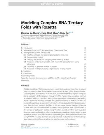
ARTICLE IN PRESS44Clarence Yu Cheng et al.using the extract lowscore decoys.py script (see also below). The preassembled helices are generally nearly identical except for small variationsnear the ends (Fig. 3). Sampling the helices in the target RNA from thesemodels instead of from the database of RNA fragments used for global sampling allows a greater portion of the computational effort to be spent on nonhelical regions.3.3. Defining the global fold using fragment assembly of RNAWith experimental constraints and preassembled helices in hand, the globalfold of the target RNA can be tackled. At this stage, we create a set of lowresolution models using Fragment Assembly of RNA (FARNA) (Das &Baker, 2007). In FARNA, models are assembled using small RNA fragments sampled from a crystallographic database using a Monte Carlo algorithm. This heuristic allows the models to take on RNA-like conformationsFigure 3 Preassembled helices for F. nucleatum double glycine riboswitch ligandbinding domain. The secondary structure is shown at center with the residues usedfor helix preassembly highlighted in color. Ensembles of 10 models of each helix generated by the helix preassembly protocol in Rosetta are shown at the periphery, labeledwith the aptamer and helix number (e.g., Apt1 P1 for the P1 helix of aptamer 1). Themagnified view of the Apt1 P1 helix highlights the slight differences in conformationbetween the preassembled helix models.

ARTICLE IN PRESSModeling Complex RNA Tertiary Folds with Rosetta45because the fragments are drawn from RNAs of known structure. Thislow-resolution modeling step does not include any refinement at the atomiclevel, because the all-atom energy landscape is too “rugged”; that is, it contains many energy minima that can trap the nascent model from exploringalternative conformations, and strategies for searching this landscape(Sripakdeevong et al., 2011) are currently too computationally expensivefor RNA domains above 10–20 nucleotides.For the following steps, if a comparison to a crystallographic or other reference model is desired, inputting the reference during the modeling runswill allow root mean square deviation (RMSD) values to be reported inthe output silent files. To properly calculate RMSDs, reference modelsmust have the same sequence as the construct being modeled. Themake rna rosetta ready.py command reformats PDB files with the correctsequence to be used as reference models (Appendix, command line [4]). Forthe glycine riboswitch example described in this chapter, the crystallographic structure includes a protein-binding loop that is not present inthe construct used for experiments and modeling. To prepare the crystallographic structure for use as a reference model, we replace the proteinbinding loop with a UUUA tetraloop to match the target sequence(Appendix, command lines [5] through [14]). These commands can alsobe used for more extensive remodeling of models and are described in detailin Section 3.6. We note that including a reference model is not required forthe modeling workflow but can allow for easy visualization of modelingresults through energy versus RMSD plots, such as those shown in Fig. 4.As with the helix assembly runs above, a series of text files will record thecommand lines used for setup and modeling. To set up a FARNA run, wecreate a file called README SETUP, which calls a script calledrna denovo setup.py to generate the command line for low-resolutionmodeling. Command line [15] in the Appendix shows an exampleREADME SETUP file. Special tags can be used to specify advanced options forthe modeling run, including specific noncanonical base pairs (Appendix),segments of the RNA that are thought to form a tertiary contact, or soft constraints from MOHCA-seq experiments. For example, to incorporate theMOHCA-seq data into computational modeling in Rosetta, a smoothpseudoenergy potential is applied between pairs of nucleotides showingstrong MOHCA-seq signal, which indicates that they are proximal in the3D fold. Two separate pseudoenergy potential functions are used, one forstrong and one for weak MOHCA-seq hits (Fig. 2E); these potentials differ

ARTICLE IN PRESS46Clarence Yu Cheng et al.Figure 4 Low-resolution modeling and full-atom refinement using FARNA and FARFAR.(A) Rosetta energy score versus RMSD plot after low-resolution modeling using FARNA.(B) Overlaid 10 lowest-energy models after low-resolution modeling using FARNA.Chain breaks are visible in many models (arrows), and residues commonly adopt unrealistic geometries. (C) Rosetta energy score versus RMSD plot after minimization usingthe FARFAR algorithm. (D) Overlaid 10 lowest-energy models after minimization usingthe FARFAR algorithm. The models do not show any chain breaks, and poor residuegeometries are greatly reduced.only in the amplitude of the energy penalty applied for residues that are tooclose or too far apart. These potentials are specified in text-formatted files inRosetta’s “constraint file” format (example in Appendix, file [F3]) and canbe input to rna denovo setup.py. The command source README SETUP(Appendix, command line [16]) generates a file containing a command linefor rna denovo with the tags given in README SETUP, called README FARFAR(Appendix, command line [17]), as well as parameter and FASTA files.It is a good idea to test the run locally before submitting it as a job to acluster, in case the run is stopped by an error. To test the run, we use sourceREADME FARFAR (Appendix, command line [18]) to begin a single job on alocal computer and wait until sampling begins successfully (command lineoutput similar to “Picked Fragment Library for sequence u and sec. struct

ARTICLE IN PRESSModeling Complex RNA Tertiary Folds with Rosetta47H . . . found 2308 potential fragments”)before canceling the run. Then perform modeling on a computer cluster by first using the rosetta submit.pyscript to generate submission files (Appendix, command line [19]) and thenusing source on the submission file appropriate for the cluster’s queuing system (e.g., Condor, LSF, PBS, etc.). For FARNA runs, it is best to generatearound 10,000–15,000 low-resolution models, from which a subset willlater be minimized. The models generated by rna denovo are by defaultplaced in a folder named out, which is created in the modeling folder.The out folder contains individual folders for each run with a silent .out filein each that describes all of the models from that run. To collect all of themodels into a single silent file, we use the easy cat.py script (Appendix,command line [20]). This creates a single concatenated .out file with thename tag initially provided in README SETUP.If a reference (native) model was input during FARNA modeling, theRMSDs of the FARNA models to the reference can be compared to theirRosetta energy scores, which are all recorded in the concatenated silent file,to assess the quality of the low-resolution models. An example energy versusRMSD plot is shown in Fig. 4A. Additionally, it may be helpful to visualizethe low-resolution models with the lowest—that is, most favorable—Rosetta energy scores. To do this, we extract the lowest-scoring modelsfrom the concatenated .out file using extract lowscore models.py(Appendix, command line [21]). These PDB-formatted models can thenbe loaded in PyMOL for comparison (Fig. 4B). Note that the FARNAmodels may contain discontinuities in the RNA backbone, which are visiblein PyMOL. These chainbreaks occur because crystallographic fragments thatare sampled and built into the model first may prevent a continuous backbone from being built in other regions of the RNA. Chainbreaks are not acause for concern, however, because the following all-atom minimizationstep typically resolves them.3.4. Producing and selecting models with reasonablestereochemistry using refinementAs mentioned earlier, the low-resolution models generated by FARNA maycontain chainbreaks and unrealistic atomic-level geometries due to themethod of sampling rigid fragments of crystallographic RNA structures.To achieve more realistic models of the RNAs, we use the rna minimizeprogram in Rosetta to refine the lowest-energy 1/6 of the low-resolutionmodels (e.g., if 12,000 FARNA models were generated, minimize 2000of them). This FARNA with Full-Atom Refinement (FARFAR) strategy

ARTICLE IN PRESS48Clarence Yu Cheng et al.optimizes the low-resolution models based on the Rosetta full-atom energyfunction, which accounts for physical and chemical features such as van derWaals forces, hydrogen bonding, desolvation penalties for polar groups, andRNA backbone torsion angles (Das et al., 2010; Sripakdeevong et al., 2011).To set up refinement of the FAR

dent 3D modeling and design of RNAs with high spatial resolution. An important driver of recent innovation has been the establishment of blind prediction trials, proposed during a community-wide collation of 3D RNA modeling methods in 2010 (Sripakdeevong, Beauchamp, & Das, 2012) and begun soon thereafter. The RNA-Puzzles trials (Cruz et al.,