WIXLIB

This article has been accepted for inclusion in a future issue of this journal. Content is final as presented, with the exception of pagination.2computational burden of optimizing the motion state over afuture horizon from a current time step. Therefore, in practical applications, these methods usually follow a recedinghorizon pattern with a limited horizon length in a schemealso known as model predictive control (MPC). These usefast real-time solvers [13], [14] to periodically solve theoptimization problems, where only a first section (step) ofthe input trajectory is executed and the process is repeatedin receding prediction horizons. MPC, which initially wasapplied to modeling human-driver like control in varioustraffic situations [15], it now appears in many works as areactive planner for autonomous and semi-autonomous vehiclecontrol [16]–[19]. To apply MPC for trajectory planningrequires the knowledge of global route waypoints as referencesto follow. For the on-road scenario, the centerline of eachlane from the perception or map information [20], [21] canbe used as the reference path. For off-road scenarios, thismethod can be incorporated in the path tracking level the pathvelocity decomposition methods [22]. In addition, specificterminal costs and constraints could be designed to circumventlimitations of robustness and stability that arise from the useof finite horizons [23], [24].In MPC-based trajectory planning, the expected states ofthe autonomously controlled vehicle (ACV or ego vehicle)and other object vehicles (OVs) are model-predicted for theduration of the prediction horizon based on the current measurements. This allows the ACV to assess the risk of havinga collision with other OVs and then to determine a collisionfree trajectory. Different models used for motion predictionof OVs are summarized in [25], including physics-basedmodels, maneuver-based models, and interaction-aware models. Physics-based models [26], [27] simply assume constantvelocity or constant accelerations and thus they can only beused in motion prediction for a short-term (less than 1 second).Maneuver-based models [28], [29] predict the motion based onthe estimation of maneuver intentions. Interaction-aware models [30], [31] also consider the inter-dependencies between theindividual vehicles’ maneuvers. The latter two models allowlonger-term prediction compared to physics-based models. Theinteraction-aware model is more reliable than maneuver-basedmodels, but it’s also much-more computationally expensive,difficult to fully characterize, and is not compatible for realtime risk assessment [25]. Maneuver-based models remain theviable options for real-time long-term motion prediction (morethan a second).The planning problem naturally involves uncertainties dueto modeling errors, sensor imperfections, or environmentaldisturbances, as summarized in [32]. In prediction of themotion of the OVs for risk assessment, the uncertainties can behandled by either using robust reachability analysis [33]–[36](estimating the propagation of the uncertainty bounds) or usingstochastic reachability analysis [37], [38] (estimating the propagation of the uncertainty distribution). In the reachabilityanalysis case, the worst case of the uncertainty is consideredthus leading to a very conservative solution for the planning problem. However, for stochastic reachability analysis,the reachable set as well as the risk of collision can beassessed by probabilities. If the state uncertainties are GaussianIEEE TRANSACTIONS ON INTELLIGENT TRANSPORTATION SYSTEMSdistributed, the stochastic reachability analysis can be implemented via filtering techniques, e.g., Kalman filter (KF)series [39], [40] for motion prediction of one maneuver andInteractive Multi Model (IMM) KF or Switching KF [41]for different possible maneuvers. Therein, the computationalprocess for solving for the collision-free trajectory of the ACVin the MPC with filtering techniques is similar to applyingstochastic reachability analysis applied to find a fail-safetrajectory [38].Also, due to the sub-optimality caused by the nonconvexconfiguration space, an ACV with static or pre-configuredoptimization setups could get trapped at undesired local minima. Therefore in [42], a predictive control framework whichcan switch from a combination of rule-based discrete maneuver decisions is applied. With these rule-based decisions,the planned trajectories can be forced out of undesired localminima. Later in [43], to improve the optimality of the maneuver decisions, the lane selection and the related desired speedselection on the lane, is integrated within the optimizationproblem. To transform the resulting mixed-integer nonlinearprogramming problem (MINP) into a regular nonlinear programming (NLP) problem for real-time implementation, weproposed a relaxation method. However, in [43], only onemaneuver can be selected for the whole prediction horizon.Furthermore, in the limited work presented there, measurementnoise and other uncertainties were not considered in theproblem formulation.The present paper builds on the above with the following additional contributions: 1) The maneuver selection isextended from searching for one optimized maneuver for theentire prediction horizon to solving for an optimized sequenceof maneuvers for the prediction horizon. Therein, a predictivereference speed assignment and adjustment strategy is proposed to pre-plan the longitudinal motion and to force theoptimization solver “jump” out of undesired minima. 2) Here,we explicitly include uncertainties in the estimation and prediction of the states of the ACV and of the OVs as well as indetermining the evolution of the tightened MPC constraintsto explicitly accommodate uncertainties. 3) We include acomputational complexity analysis of the naive MINP formulation as well as of the proposed relaxation technique for thespecific active set solver adopted. 4) We compare the performance of the proposed optimized maneuver sequence planningwith the one optimized maneuver approach under extendedsimulations that covers several complex scenarios on ahighway.The rest of the paper is organized as follows. Section IIintroduces the overall control framework. Section III describesthe vehicle model of the ACV and the OV subject to sensing uncertainty and filtering techniques for state estimationand prediction. The hybrid system modeling of the vehiclemaneuvers as well as the rule-based reference speed automatonare given in Section IV. Section V describes the formulationof MPC for maneuver and trajectory planning, the relaxationmethod proposed to transform the MINP to NLP and thereduction of the computational complexity due to the proposed relaxation. Simulations results and corresponding discussions are included in Section VI to illustrate the workings

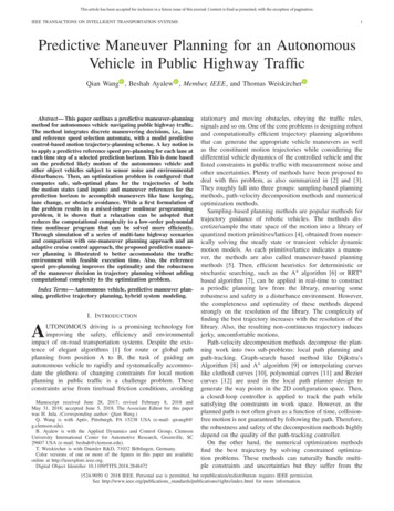
This article has been accepted for inclusion in a future issue of this journal. Content is final as presented, with the exception of pagination.WANG et al.: PREDICTIVE MANEUVER PLANNING FOR AN AUTONOMOUS VEHICLE IN PUBLIC HIGHWAY TRAFFICFig. 2.Fig. 1.Hierachical control framework.of the proposed framework. Conclusions are offered inSection VII.II. C ONTROL F RAMEWORKFigure 1 shows a schematic of the proposed predictivemaneuver planning and control framework for an autonomousroad vehicle in a uncertained public traffic environment. At thetop the assigner module integrates/fuses the information fromthe environment perception module (lane detection, trafficsign and signals, object tracking. . .), the navigator/path planner module (route navigator for on-road situation and pathplanner for off-road situation), the vehicle dynamics sensing/estimation modules (planer and yaw motion of the ACV)and motion prediction module (both ACV and tracked OVs).Here, we assume the states of the ACV x a and OV x o are fullyobserved/estimated. The fused information will be providedto some pre-defined finite state machines (FSMs)/maneuverautomatons and then the decisions on configurations, e.g.,parameters ( p), references (r ), and constraints (c), for theMPC formulation will be made and assigned to the predictivetrajectory guidance (PTG) module. Further description of thesecan be found in [19] and will be also briefly mentioned inSection III.The maneuver automatons/FSMs designed and stored inthe assigner module are scenario-based. Once the possiblemaneuvers for a scenario are captured, like cruising, following,leading and lane change for highway scenario [44] (seeFigure 4), or going left/right/straight and stop for intersectionscenario [45], the relevant FSM can be easily extended forthe same scenario or to other scenarios [46]. The candidatemaneuvers in the FSMs are related to their own references,e.g. desired speed and lane. At each prediction interval ofthe MPC, the references are pre-selected according to thepredicted motion of the ACV and the surrounding OVs viafiltering techniques. Then, the optimized maneuver sequenceas well as the optimized relevant control output trajectory ufor the whole horizon are solved simultaneously by the PTG3Particle motion description for the vehicle.system, according to the objective function and constraints tobe detailed later. When the maneuver planning is done, the firstinterval of u, i.e., u 0 is sent to the lower-level controllers of thecontinuous vehicle dynamics for execution via the availablelower-level vehicle dynamics controllers (VDC). The lowerlevel controllers are responsible for manipulating the availableactuators like electronic throttle, braking actuators or electricsteering motors so as to track the desired longitudinal andlateral acceleration signals generated by the upper-level PTGsystem. The reader is referred to [19], [47] and other standardreferences for this topic.III. V EHICLE M ODELS AND F ILTERING D ESIGNA. Particle Motion Based Vehicle ModelThe use of a 2D curvilinear particle motion model inthe Frenet frame (see Figure 2) for vehicle motion description in trajectory planning has been detailed in previousworks [19], [48]. The reasons we adopted this model include:1) it is simple enough to use and implement for real-timecomputations, 2) it describes the kinematic planar motionof an object like a car well, 3) we can incorporate roadcurvature information directly in the model; thus, it is suitablefor path tracking problems. For convenience, we shall presenthere the continuous time models of the state dynamics evenif computations are ultimately to be done in discrete timeform. Adding process uncertainties (random disturbances anduncertainties) and measurement noise, the nonlinear dynamicmodel describing the motion of the ACV can be written as: atv̇ t ψ̇e ψ̇ p v t cos(ψe )κ(s)/[1 ye κ(s)] ṡ v t cos(ψe )/[1 ye κ(s)] ẏe vsin(ψ)te ȧt at /Tat[vκ(s) ψ̇]/Tψ̈ ptpψ̇ p 000 0 0 0 00 0 0 wat at,d 00 0 0 w ψ̇ 00 ψ̇ p,d d 1 0 1/Tat0 01/Tψ̇ p0 1

This article has been accepted for inclusion in a future issue of this journal. Content is final as presented, with the exception of pagination.4IEEE TRANSACTIONS ON INTELLIGENT TRANSPORTATION SYSTEMS ys0 y ye 0 ya t 0yψ̇ p0 1 0 0000001000010001000010 vt 0 0 ψe s 0 0 1 0 ye 0 1 at ψ̇ p vs0 v ye 0 0 v at v ψ̇ p1 01 1 K s2 00 (1)where v t , at and ψ̇ p are, respectively, the absolute forwardspeed, forward acceleration and yaw rate of the vehicle. ψe ,s and ye are, respectively, the angular alignment error, arclength and lateral position error of the vehicle with respect tothe reference path coordinate. The reference path is definedby its curvature κ(s) in terms of the arc length s. κ(s) can becaptured by interpolating curves, e.g., polynomial curves bylane detection [20], [21] from perception module or from apath planning module [11]. In addition, assuming the (lowerlevel) closed-loop vehicle dynamics exhibits a first-order lagbehavior, the generation of at and ψ̇ p can be approximated bya first-order dynamics system with additive Gaussian processnoise w [wat w ψ̇d ]. This process noise is used to modeldisturbances (e.g. wind, road, unmolded dynamics) affectingthe longitudinal and lateral dynamics of the ACV. Tat , Tψ̇ pare the time-constants of the first-order approximation ofthe longitudinal and lateral dynamics of the vehicle (maskedby available VDC). Here, the desired forward accelerationat,d and the desired deviation from the reference yaw rate ψ̇ p,d are treated as the final inputs used to control thevehicle/particle along the reference path. The use of ψ̇ p,dfacilitates the computation of smooth inputs since knownreference curvature information is already taken into account(see [19]). For the system outputs, we consider that theavailable measurements are positions s, ye (e.g., from GPS)and the inertial states at , ψ̇ p (e.g., from IMU) with assumedGaussian sensor noise v [v s v ye v at v ψ̇ p ]T .For an OV, its motion is also defined in the Frenet frameas a particle. To consider its maneuver intention for bettermotion prediction, we assume each OV to follow closed-formdynamics that describe longitudinal motion like cruising at aspecific speed or speed change and lateral motion like tackinga specific lane or lane change. One possible form is: 0 100soṡo K s1 s s v̇ t,o000 v t,o 1 Ks2 ye,o ẏe,o 0001 ssv̇ n,ov n,o00 K y1 K y2 00 s K s10 v t,o,re f 1 K s2 y e,o,ref000K y1 ys oy ye,o 1000010 0 wṡ,o w y,o0 1 so s 0 v t,o 100 ye,o sv n,o01 v s,ov y,o(2)where, so and ye,o are the arc length and lateral position errors and v sof the OV; v t,on,o are the tangential speed and normalspeed of the OV along its reference lane. K s1 and K s2 are theproportional and integral gains of a controlled OV trackingsthe reference speed v t,o,ref with assumed Gaussian processnoise wṡ,o . K y1 and K y2 are the proportional and integralgains of a controlled OV tracking its reference lane ye,o,re fwith assumed Gaussian process noise w y,o . These gains canbe identified from the human-driver data to emulate differentdriving habits, e.g. either aggressive or conservative [49]. Forsystem outputs, only the positions so and ye,o are assumedmeasured with associated Gaussian sensor noises v s,o and v y,o(e.g., from on-board range sensors like radars on the ACV).B. Filtering Design for Motion Estimation and PredictionGiven the nonlinear system model in (1), we adoptUnscented Kalman Filter (UKF) [50] to estimate the motionstates of ACV in the presence of process and measurementuncertainty/noise. Given the linear dynamics motion modelsfor the OVs (2), a regular KF can be used for state estimationof one maneuver (tracking a specific lane and speed). Toaccount for other possible maneuvers of the OVs, the Interactive Multi-Model KF algorithm [41], [51] can be appliedfor OV state estimation. Here, we assume the gains are wellcaptured from the driving data for the drivers of all OVs ofall maneuvers.Given the current estimates of the ACV and OV states,one can predict the evolution of the mean and covarianceof the states for the whole length of the prediction horizon of the MPC. Here, we propagate uncertainty in thepredicted states (for both ACV and OV) using the filteringtechniques(UKF/KF) based on (1) and (2) with the notionof the most likely measurement. This notion is based on theassumption that the future measurements in the update of thefilter recursions are approximated well by the prediction. Thisassumption is motivated by the fact that future measurementsare unavailable. Even though the updated covariance is notdirectly affected by the value of the measurement, as the measurement information is considered (via the only assumptionthat same sensors and models are to be used), the uncertaintiesin the likely state are reduced. It is shown in [39] that the mostlikely measurement will not introduce bias in the system, thusit is useful to constrain the uncertainty propagation. Finally,note that the future inputs used in the motion prediction ofthe ACV will be taken from the previous planning results ofthe MPC.

This article has been accepted for inclusion in a future issue of this journal. Content is final as presented, with the exception of pagination.WANG et al.: PREDICTIVE MANEUVER PLANNING FOR AN AUTONOMOUS VEHICLE IN PUBLIC HIGHWAY TRAFFIC5The above models for motion prediction of OVs and theACV do not explicitly consider the interactions between vehicles, particularly those that would exist in mixed-traffic involving other human-driven vehicles. As alternatives, other motionprediction approaches such as interactive multi-model filtering,Bayesian Networks, and Hidden Markov Models trained onhuman-driver data are all possible options [31], [52]. Whileany of these approaches may be used for motion prediction andincorporated with the maneuver planning framework presentedin this paper, as we point out later, for multiple OVs in multilane scenarios, the computational complexity of using evenlinear motion models for the OVs needs to be handled withcare.IV. H YBRID S YSTEM M ODELING OF THE V EHICLEM ANEUVERS AND RULE -BASED R EFERENCES PEED AUTOMATONA. Hybrid System Modeling of the Vehicle ManeuversThe hybrid system notion is straightforward to apply tothe motion of a road vehicle, since basic maneuvers, likeaccelerating, cruising or decelerating in the longitudinal direction and steering to the left or right in the lateral directioncan be identified from the vehicle’s motion [44], [45]. Forthe ACV, these maneuvers can be designed via trackingdifferent reference speeds and reference paths/lanes [42]. Thisresults in a hybrid system model involving tracking of twodimensional discrete references (speed and lane) and theunderlying continuous vehicle motion trajectories. To reducethe complexity of the maneuver planning for a predictionhorizon, the switching among the discrete references can bedone hierarchically (see Figure 3, for example): 1) Firstly,the switching of the reference speeds assigned for each lanebased on pre-defined rules (rule-based switch sets) is executedat each prediction step in the horizon. This is called rule-basedswitch. 2) Then, an optimization problem is solved for thewhole horizon to find the optimized switching sequence for thereference lanes. This is called optimization-based switch. Fordifferent scenarios, the maneuvers and the rule-based switchsets can be specifically designed and stored in different FSMsof the assigner module, e.g., single lane, intersection, etc.B. Rule-Based Reference Speed Automaton1) Reference Speed Assignment: Considering the interactionof the vehicle with the surrounding dynamic environment,e.g. the traffic sign, signals and OVs, for example, whenapproaching a slow front OV, a normal reaction of the vehiclewill be either slowing down to follow it or simply changinglane to overtake it. Those intentions can be reflected by thereference speed assignment to the ACV. Specifically, on lanel, a relevant reference speed v t,r,l will be assigned to the ACVto follow, depending on the detection of approaching or closeby object vehicles, as shown in Figure 4. The detectioncondition (3) and approaching condition (4) are defined by:ŝ ŝoi Td v t,re fŝ ŝoisv t,re f v̂ t,o 0i(3)(4)Fig. 3.Maneuver automaton example for 3-lane highway scenario.Rule-based switch sets are denoted by R.where Td is the detection preview time (set from specificationsof the perception module, its value should be larger than thepredictive horizon H p to prevent the ignorance of an abruptevent from the surrounding traffic for MPC). Here, and inthe following, the usual hat ( ) notation is used to denote therespective estimated states. The i t h OV occupying lane l isdenoted by: ŷe,oi ye,l , ye,l(5)where ye,oi is the lateral position of OV i in the path coordinateand the lanel is demarked by the lateral position bounds ye,l , ye,l .Accordingly, the cruising maneuver is defined as trackinga desired cruise speed v t,re f on lane l (lane 2 in Figure 4)without detecting any approaching OVs on the same lane. Thecorresponding speed relation and reference speed assignmentis given by:v t,r,l v t,re f(6)The following or leading maneuver refers to tracking thesspeed v t,oiof a detected approaching OV on lane l in thefront or rear by assigning:sv t,r,l v̂ t,oi(7)2) Reference Speed Adjustment: Generally, the ACV isexpected to track the desired cruise speed v t,re f withinthe acceptable speed range [v t,cl , v t,ch ] with positive speed

This article has been accepted for inclusion in a future issue of this journal. Content is final as presented, with the exception of pagination.6Fig. 4.IEEE TRANSACTIONS ON INTELLIGENT TRANSPORTATION SYSTEMSReference speed assignment for ACV in 2 lane scenario.tolerance v t : v t,cl v t,re f v tv t,ch v t,re f v tFig. 5.Prediction of reference speed assignment and adjustment.TABLE I(8)However, as argued in [43], by following the optimizationbased reference lane automaton introduced in the next section,the ACV can be “trapped” in one lane in a following or leadingmaneuver due to the formulation of MPC objective functionwith a lane selection variable (to be described later). In suchsituations, a forced lane change is necessary to help the ACVjump out of the trap. Therefore, we extend the rules usedin [42] to guide the ACV to an adjacent empty lane or to onewith the assigned speed closest to the desired cruise speed viareference speed adjustment. If the assigned reference speed ofthe ACV in the current lane l goes outside of this speed range: (9)/ v t,cl , v t,chv̂ t,r,l and adjacent lane(s) are unoccupied or are with assignedspeeds closest to v t,re f , with complementary sets defined by: / v t,cl , v t,chŝ ŝotl ds or v̂ t,r,l 1 or v̂ t,r,l 1 v t,re f min v̂ t,r,i v t,re f , i [1, . . . , Nl ](10)then a forced lane change will be assigned. Here, ds is a safeheadway distance between the ACV and the preceding OVwhich will be defined in the next section (see equation (13)).A forced lane change is activated by adjusting the assignedspeed for those lanes with following or leading maneuveroutside the acceptable speed range. The adjustment is givenby: v t,maxss,k,v̂ /v,v 0, s(11)v t,r, j kl v̂ t,ot,cl t,chlt,o jjv̂ t,oiwhere kl is the adjustment factor and v t,max is the maximumspeed of the ACV. kl can be selected to generate a highvalue of the objective function associated with tracking theC ONFIGURATION OF THE RULE -BASED R EFERENCES PEED AUTOMATON FOR L ANE ladjusted reference speed of specific lanes. This will then forcethe MPC to track other lanes with closer assigned referencespeed to the desired cruising speed v t,re f with lower valuesof the objective function. An example of the reference speedassignment and adjustment for multiple-lane scenario is shownin Figure 5.In summary, the configurations of rule-based referencespeed automatons for FSMs are listed as in Table I. In therule description, the symbol “ ” represents intersection, “ ”means union, and the superscript “C” represents complement.Remark 1: Given a prediction horizon of length N p steps,the rule-based reference speed automaton of Table 1 is appliedfor every lane at every prediction interval. This means areference speed sequence with N p elements will be generatedfor each lane, thus effectively constructing a two-dimensionalpre-plan of the references in both the longitudinal and lateraldirections. This will be used later in the MPC to find the bestsequence of reference selections for the whole horizon thatminimize an objective function. Note that there is a possibleloss of performance from the non-optimality of the referencespeed assignment rules; but these are discrete rules executedoutside of the MPC; the optimization of such assignment rulesis beyond the scope of our

also known as model predictive control (MPC). These use fast real-time solvers [13], [14] to periodically solve the optimization problems, where only a first section (step) of the input trajectory is executed and the process is repeated in receding prediction horizons. MPC, which initially was applied to modeling human-driver like control in .