Transcription
XGBoost: A Scalable Tree Boosting SystemTianqi ChenCarlos GuestrinUniversity of WashingtonUniversity of Washingtontqchen@cs.washington.eduABSTRACTTree boosting is a highly effective and widely used machinelearning method. In this paper, we describe a scalable endto-end tree boosting system called XGBoost, which is usedwidely by data scientists to achieve state-of-the-art resultson many machine learning challenges. We propose a novelsparsity-aware algorithm for sparse data and weighted quantile sketch for approximate tree learning. More importantly,we provide insights on cache access patterns, data compression and sharding to build a scalable tree boosting system.By combining these insights, XGBoost scales beyond billionsof examples using far fewer resources than existing systems.KeywordsLarge-scale Machine Learning1.INTRODUCTIONMachine learning and data-driven approaches are becoming very important in many areas. Smart spam classifiersprotect our email by learning from massive amounts of spam data and user feedback; advertising systems learn tomatch the right ads with the right context; fraud detectionsystems protect banks from malicious attackers; anomalyevent detection systems help experimental physicists to findevents that lead to new physics. There are two important factors that drive these successful applications: usage ofeffective (statistical) models that capture the complex datadependencies and scalable learning systems that learn themodel of interest from large datasets.Among the machine learning methods used in practice,gradient tree boosting [10]1 is one technique that shinesin many applications. Tree boosting has been shown togive state-of-the-art results on many standard classificationbenchmarks [16]. LambdaMART [5], a variant of tree boosting for ranking, achieves state-of-the-art result for ranking1Gradient tree boosting is also known as gradient boostingmachine (GBM) or gradient boosted regression tree (GBRT)Permission to make digital or hard copies of all or part of this work for personal orclassroom use is granted without fee provided that copies are not made or distributedfor profit or commercial advantage and that copies bear this notice and the full citation on the first page. Copyrights for components of this work owned by others thanACM must be honored. Abstracting with credit is permitted. To copy otherwise, or republish, to post on servers or to redistribute to lists, requires prior specific permissionand/or a fee. Request permissions from permissions@acm.org.KDD ’16, August 13-17, 2016, San Francisco, CA, USAc 2016 ACM. ISBN 978-1-4503-4232-2/16/08. . . 15.00DOI: cs.washington.eduproblems. Besides being used as a stand-alone predictor, itis also incorporated into real-world production pipelines forad click through rate prediction [15]. Finally, it is the defacto choice of ensemble method and is used in challengessuch as the Netflix prize [3].In this paper, we describe XGBoost, a scalable machinelearning system for tree boosting. The system is availableas an open source package2 . The impact of the system hasbeen widely recognized in a number of machine learning anddata mining challenges. Take the challenges hosted by themachine learning competition site Kaggle for example. Among the 29 challenge winning solutions 3 published at Kaggle’s blog during 2015, 17 solutions used XGBoost. Amongthese solutions, eight solely used XGBoost to train the model, while most others combined XGBoost with neural nets in ensembles. For comparison, the second most popularmethod, deep neural nets, was used in 11 solutions. Thesuccess of the system was also witnessed in KDDCup 2015,where XGBoost was used by every winning team in the top10. Moreover, the winning teams reported that ensemblemethods outperform a well-configured XGBoost by only asmall amount [1].These results demonstrate that our system gives state-ofthe-art results on a wide range of problems. Examples ofthe problems in these winning solutions include: store salesprediction; high energy physics event classification; web textclassification; customer behavior prediction; motion detection; ad click through rate prediction; malware classification;product categorization; hazard risk prediction; massive online course dropout rate prediction. While domain dependent data analysis and feature engineering play an importantrole in these solutions, the fact that XGBoost is the consensus choice of learner shows the impact and importance ofour system and tree boosting.The most important factor behind the success of XGBoostis its scalability in all scenarios. The system runs more thanten times faster than existing popular solutions on a singlemachine and scales to billions of examples in distributed ormemory-limited settings. The scalability of XGBoost is dueto several important systems and algorithmic optimizations.These innovations include: a novel tree learning algorithmis for handling sparse data; a theoretically justified weightedquantile sketch procedure enables handling instance weightsin approximate tree learning. Parallel and distributed computing makes learning faster which enables quicker model exploration. More importantly, XGBoost exploits ons come from of top-3 teams of each competitions.
computation and enables data scientists to process hundredmillions of examples on a desktop. Finally, it is even moreexciting to combine these techniques to make an end-to-endsystem that scales to even larger data with the least amountof cluster resources. The major contributions of this paperis listed as follows: We design and build a highly scalable end-to-end treeboosting system. We propose a theoretically justified weighted quantilesketch for efficient proposal calculation. We introduce a novel sparsity-aware algorithm for parallel tree learning. We propose an effective cache-aware block structurefor out-of-core tree learning.Figure 1: Tree Ensemble Model. The final prediction for a given example is the sum of predictionsfrom each tree.it into the leaves and calculate the final prediction by summing up the score in the corresponding leaves (given by w).To learn the set of functions used in the model, we minimizethe following regularized objective.XXL(φ) l(ŷi , yi ) Ω(fk )While there are some existing works on parallel tree boosting [22, 23, 19], the directions such as out-of-core computation, cache-aware and sparsity-aware learning have notbeen explored. More importantly, an end-to-end systemthat combines all of these aspects gives a novel solution forreal-world use-cases. This enables data scientists as well asresearchers to build powerful variants of tree boosting algorithms [7, 8]. Besides these major contributions, we alsomake additional improvements in proposing a regularizedlearning objective, which we will include for completeness.The remainder of the paper is organized as follows. Wewill first review tree boosting and introduce a regularizedobjective in Sec. 2. We then describe the split finding methods in Sec. 3 as well as the system design in Sec. 4, includingexperimental results when relevant to provide quantitativesupport for each optimization we describe. Related workis discussed in Sec. 5. Detailed end-to-end evaluations areincluded in Sec. 6. Finally we conclude the paper in Sec. 7.Here l is a differentiable convex loss function that measuresthe difference between the prediction ŷi and the target yi .The second term Ω penalizes the complexity of the model(i.e., the regression tree functions). The additional regularization term helps to smooth the final learnt weights to avoidover-fitting. Intuitively, the regularized objective will tendto select a model employing simple and predictive functions.A similar regularization technique has been used in Regularized greedy forest (RGF) [25] model. Our objective andthe corresponding learning algorithm is simpler than RGFand easier to parallelize. When the regularization parameter is set to zero, the objective falls back to the traditionalgradient tree boosting.2.2.2TREE BOOSTING IN A NUTSHELLWe review gradient tree boosting algorithms in this section. The derivation follows from the same idea in existingliteratures in gradient boosting. Specicially the second ordermethod is originated from Friedman et al. [12]. We make minor improvements in the reguralized objective, which werefound helpful in practice.2.1iŷi φ(xi ) KXGradient Tree BoostingL(t) fk (xi ), fk F ,nXl(yi , yˆi (t 1) ft (xi )) Ω(ft )i 1This means we greedily add the ft that most improves ourmodel according to Eq. (2). Second-order approximationcan be used to quickly optimize the objective in the generalsetting [12].(1)k 1L(t) 'm(2)The tree ensemble model in Eq. (2) includes functions asparameters and cannot be optimized using traditional optimization methods in Euclidean space. Instead, the model(t)is trained in an additive manner. Formally, let ŷi be theprediction of the i-th instance at the t-th iteration, we willneed to add ft to minimize the following objective.Regularized Learning ObjectiveFor a given data set with n examples and m featuresD {(xi , yi )} ( D n, xi Rm , yi R), a tree ensemble model (shown in Fig. 1) uses K additive functions topredict the output.k1where Ω(f ) γT λkwk22Twhere F {f (x) wq(x) }(q : R T, w R ) is thespace of regression trees (also known as CART). Here q represents the structure of each tree that maps an example tothe corresponding leaf index. T is the number of leaves in thetree. Each fk corresponds to an independent tree structureq and leaf weights w. Unlike decision trees, each regressiontree contains a continuous score on each of the leaf, we usewi to represent score on i-th leaf. For a given example, wewill use the decision rules in the trees (given by q) to classifynX[l(yi , ŷ (t 1) ) gi ft (xi ) i 11hi ft2 (xi )] Ω(ft )2where gi ŷ(t 1) l(yi , ŷ (t 1) ) and hi ŷ2(t 1) l(yi , ŷ (t 1) )are first and second order gradient statistics on the loss function. We can remove the constant terms to obtain the following simplified objective at step t.L̃(t) nXi 1[gi ft (xi ) 1hi ft2 (xi )] Ω(ft )2(3)
Algorithm 1: Exact Greedy Algorithm for Split FindingInput: I, instance set of current nodeInput: d, feature dimensiongain P0PG i I gi , H i I hifor k 1 to m doGL 0, HL 0for j in sorted(I, by xjk ) doGL GL gj , HL HL hjGR G GL , H R H H LG2G2G2score max(score, HLL λ HRR λ H λ)endendOutput: Split with max scoreFigure 2: Structure Score Calculation. We onlyneed to sum up the gradient and second order gradient statistics on each leaf, then apply the scoringformula to get the quality score.Define Ij {i q(xi ) j} as the instance set of leaf j. Wecan rewrite Eq (3) by expanding Ω as followsL̃(t) nX[gi ft (xi ) i 1 T1 X 21hi ft2 (xi )] γT λwj22 j 1TXX1 Xhi λ)wj2 ] γT[(gi )wj (2j 1 i Ii IjAlgorithm 2: Approximate Algorithm for Split Findingfor k 1 to m doPropose Sk {sk1 , sk2 , · · · skl } by percentiles on feature k.Proposal can be done per tree (global), or per split(local).endfor k 1 to Pm doGkv j {j sk,v xjk sk,v 1 } gjPHkv j {j sk,v xjk sk,v 1 } hjendFollow same step as in previous section to find maxscore only among proposed splits.(4)jFor a fixed structure q(x), we can compute the optimalweight wj of leaf j byPi Ij gi P,(5)wj i Ij hi λand calculate the corresponding optimal value byP2T1 X ( i Ij gi )(t)PL̃ (q) γT.2 j 1 i Ij hi λ(6)Eq (6) can be used as a scoring function to measure thequality of a tree structure q. This score is like the impurityscore for evaluating decision trees, except that it is derivedfor a wider range of objective functions. Fig. 2 illustrateshow this score can be calculated.Normally it is impossible to enumerate all the possibletree structures q. A greedy algorithm that starts from asingle leaf and iteratively adds branches to the tree is usedinstead. Assume that IL and IR are the instance sets of leftand right nodes after the split. Lettting I IL IR , thenthe loss reduction after the split is given by" P#PP2( i IR gi )2( i I gi )21 ( i IL gi )PPPLsplit γ2i IL hi λi IR hi λi I hi λ(7)This formula is usually used in practice for evaluating thesplit candidates.2.3Shrinkage and Column SubsamplingBesides the regularized objective mentioned in Sec. 2.1,two additional techniques are used to further prevent overfitting. The first technique is shrinkage introduced by Friedman [11]. Shrinkage scales newly added weights by a factorη after each step of tree boosting. Similar to a learning ratein tochastic optimization, shrinkage reduces the influence ofeach individual tree and leaves space for future trees to improve the model. The second technique is column (feature)subsampling. This technique is used in RandomForest [4,13], It is implemented in a commercial software TreeNet 4for gradient boosting, but is not implemented in existingopensource packages. According to user feedback, using column sub-sampling prevents over-fitting even more so thanthe traditional row sub-sampling (which is also supported).The usage of column sub-samples also speeds up computations of the parallel algorithm described later.3.3.1SPLIT FINDING ALGORITHMSBasic Exact Greedy AlgorithmOne of the key problems in tree learning is to find thebest split as indicated by Eq (7). In order to do so, a split finding algorithm enumerates over all the possible splitson all the features. We call this the exact greedy algorithm.Most existing single machine tree boosting implementations, such as scikit-learn [20], R’s gbm [21] as well as the singlemachine version of XGBoost support the exact greedy algorithm. The exact greedy algorithm is shown in Alg. 1. Itis computationally demanding to enumerate all the possiblesplits for continuous features. In order to do so efficiently,the algorithm must first sort the data according to featurevalues and visit the data in sorted order to accumulate thegradient statistics for the structure score in Eq (7).3.2Approximate AlgorithmThe exact greedy algorithm is very powerful since it enumerates over all possible splitting points greedily. However,it is impossible to efficiently do so when the data does not fitentirely into memory. Same problem also arises in the et
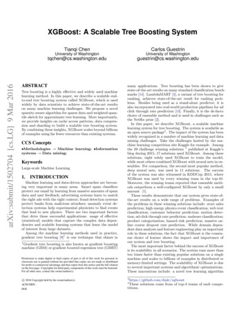
0.830.82Test AUC0.810.800.790.78exact greedyglobal eps 0.3local eps 0.3global eps 0.050.770.760.750102030405060Number of Iterations7080Figure 4: Tree structure with default directions. Anexample will be classified into the default directionwhen the feature needed for the split is missing.90Figure 3: Comparison of test AUC convergence onHiggs 10M dataset. The eps parameter correspondsto the accuracy of the approximate sketch. Thisroughly translates to 1 / eps buckets in the proposal.We find that local proposals require fewer buckets,because it refine split candidates.tributed setting. To support effective gradient tree boostingin these two settings, an approximate algorithm is needed.We summarize an approximate framework, which resembles the ideas proposed in past literatures [17, 2, 22], inAlg. 2. To summarize, the algorithm first proposes candidate splitting points according to percentiles of feature distribution (a specific criteria will be given in Sec. 3.3). Thealgorithm then maps the continuous features into buckets split by these candidate points, aggregates the statisticsand finds the best solution among proposals based on theaggregated statistics.There are two variants of the algorithm, depending onwhen the proposal is given. The global variant proposes allthe candidate splits during the initial phase of tree construction, and uses the same proposals for split finding at all levels. The local variant re-proposes after each split. The globalmethod requires less proposal steps than the local method.However, usually more candidate points are needed for theglobal proposal because candidates are not refined after eachsplit. The local proposal refines the candidates after splits,and can potentially be more appropriate for deeper trees. Acomparison of different algorithms on a Higgs boson datasetis given by Fig. 3. We find that the local proposal indeedrequires fewer candidates. The global proposal can be asaccurate as the local one given enough candidates.Most existing approximate algorithms for distributed treelearning also follow this framework. Notably, it is also possible to directly construct approximate histograms of gradientstatistics [22]. It is also possible to use other variants of binning strategies instead of quantile [17]. Quantile strategybenefit from being distributable and recomputable, whichwe will detail in next subsection. From Fig. 3, we also findthat the quantile strategy can get the same accuracy as exactgreedy given reasonable approximation level.Our system efficiently supports exact greedy for the singlemachine setting, as well as approximate algorithm with bothlocal and global proposal methods for all settings. Users canfreely choose between the methods according to their needs.3.3Weighted Quantile SketchOne important step in the approximate algorithm is topropose candidate split points. Usually percentiles of a feature are used to make candidates distribute evenly on the da-ta. Formally, let multi-set Dk {(x1k , h1 ), (x2k , h2 ) · · · (xnk , hn )}represent the k-th feature values and second order gradientstatistics of each training instances. We can define a rankfunctions rk : R [0, ) asX1rk (z) Ph,(8)h(x,h) Dk(x,h) Dk ,x zwhich represents the proportion of instances whose featurevalue k is smaller than z. The goal is to find candidate splitpoints {sk1 , sk2 , · · · skl }, such that rk (sk,j ) rk (sk,j 1 ) , sk1 min xik , skl max xik .ii(9)Here is an approximation factor. Intuitively, this meansthat there is roughly 1/ candidate points. Here each datapoint is weighted by hi . To see why hi represents the weight,we can rewrite Eq (3) asnX1hi (ft (xi ) gi /hi )2 Ω(ft ) constant,2i 1which is exactly weighted squared loss with labels gi /hi andweights hi . For large datasets, it is non-trivial to find candidate splits that satisfy the criteria. When every instancehas equal weights, an existing algorithm called quantile sketch [14, 24] solves the problem. However, there is noexisting quantile sketch for the weighted datasets. Therefore, most existing approximate algorithms either resortedto sorting on a random subset of data which have a chance offailure or heuristics that do not have theoretical guarantee.To solve this problem, we introduced a novel distributedweighted quantile sketch algorithm that can handle weighteddata with a provable theoretical guarantee. The general ideais to propose a data structure that supports merge and pruneoperations, with each operation proven to maintain a certainaccuracy level. A detailed description of the algorithm aswell as proofs are given in the supplementary material5 (linkin the footnote).3.4Sparsity-aware Split FindingIn many real-world problems, it is quite common for theinput x to be sparse. There are multiple possible causesfor sparsity: 1) presence of missing values in the data; 2)frequent zero entries in the statistics; and, 3) artifacts offeature engineering such as one-hot encoding. It is important to make the algorithm aware of the sparsity pattern inthe data. In order to do so, we propose to add a defaultdirection in each tree node, which is shown in Fig. 4. Whena value is missing in the sparse matrix x, the instance is5Link to the supplementary materialhttp://homes.cs.washington.edu/ tqchen/pdf/xgboost-supp.pdf
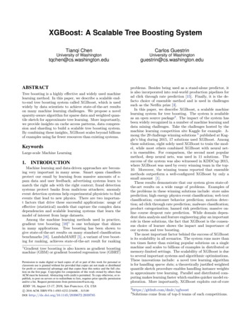
Figure 6: Block structure for parallel learning. Each column in a block is sorted by the corresponding featurevalue. A linear scan over one column in the block is sufficient to enumerate all the split points.classified into the default direction. There are two choicesof default direction in each branch. The optimal default directions are learnt from the data. The algorithm is shown inAlg. 3. The key improvement is to only visit the non-missingentries Ik . The presented algorithm treats the non-presenceas a missing value and learns the best direction to handlemissing values. The same algorithm can also be appliedwhen the non-presence corresponds to a user specified valueby limiting the enumeration only to consistent solutions.To the best of our knowledge, most existing tree learningalgorithms are either only optimized for dense data, or needspecific procedures to handle limited cases such as categorical encoding. XGBoost handles all sparsity patterns in aunified way. More importantly, our method exploits the sparsity to make computation complexity linear to numberof non-missing entries in the input. Fig. 5 shows the comparison of sparsity aware and a naive implementation on anAllstate-10K dataset (description of dataset given in Sec. 6).We find that the sparsity aware algorithm runs 50 timesfaster than the naive version. This confirms the importanceof the sparsity aware algorithm.32Basic algorithm168Time per Tree(sec)Algorithm 3: Sparsity-aware Split FindingInput: I, instance set of current nodeInput: Ik {i I xik 6 missing}Input: d, feature dimensionAlso applies to the approximate setting, only collectstatistics of non-missing entries into bucketsgain P0PG i I , gi ,H i I hifor k 1 to m do// enumerate missing value goto rightGL 0, HL 0for j in sorted(Ik , ascent order by xjk ) doGL GL g j , H L H L h jGR G GL , H R H H LG2G2G2score max(score, HLL λ HRR λ H λ)end// enumerate missing value goto leftGR 0, HR 0for j in sorted(Ik , descent order by xjk ) doGR GR gj , HR HR hjGL G GR , HL H HRG2G2G2score max(score, HLL λ HRR λ H λ)endendOutput: Split and default directions with max gain4210.5Sparsity aware algorithm0.250.1250.06250.031251284Number of Threads16Figure 5: Impact of the sparsity aware algorithmon Allstate-10K. The dataset is sparse mainly dueto one-hot encoding. The sparsity aware algorithmis more than 50 times faster than the naive versionthat does not take sparsity into consideration.4.4.1SYSTEM DESIGNColumn Block for Parallel LearningThe most time consuming part of tree learning is to getthe data into sorted order. In order to reduce the cost ofsorting, we propose to store the data in in-memory units,which we called block. Data in each block is stored in thecompressed column (CSC) format, with each column sortedby the corresponding feature value. This input data layoutonly needs to be computed once before training, and can bereused in later iterations.In the exact greedy algorithm, we store the entire datasetin a single block and run the split search algorithm by linearly scanning over the pre-sorted entries. We do the splitfinding of all leaves collectively, so one scan over the blockwill collect the statistics of the split candidates in all leafbranches. Fig. 6 shows how we transform a dataset into theformat and find the optimal split using the block structure.The block structure also helps when using the approximate algorithms. Multiple blocks can be used in this case,with each block corresponding to subset of rows in the dataset.Different blocks can be distributed across machines, or stored on disk in the out-of-core setting. Using the sortedstructure, the quantile finding step becomes a linear scanover the sorted columns. This is especially valuable for local proposal algorithms, where candidates are generated frequently at each branch. The binary search in histogram aggregation also becomes a linear time merge style algorithm.Collecting statistics for each column can be parallelized,giving us a parallel algorithm for split finding. Importantly,the column block structure also supports column subsampling, as it is easy to select a subset of columns in a block.
128166432284Number of Threads16(a) Allstate 10M841284Number of Threads1621(b) Higgs 10M0.25Basic algorithmCache-aware algorithm40.51618Basic algorithmCache-aware algorithmTime per Tree(sec)32Basic algorithmCache-aware algorithmTime per Tree(sec)6488256Basic algorithmCache-aware algorithmTime per Tree(sec)Time per Tree(sec)128210.51284Number of Threads160.251(c) Allstate 1M284Number of Threads16(d) Higgs 1MFigure 7: Impact of cache-aware prefetching in exact greedy algorithm. We find that the cache-miss effectimpacts the performance on the large datasets (10 million instances). Using cache aware prefetching improvesthe performance by factor of two when the dataset is large.128block size 2 12block size 2 16Time Complexity Analysis Let d be the maximum depthof the tree and K be total number of trees. For the exact greedy algorithm, the time complexity of original spaseaware algorithm is O(Kdkxk0 log n). Here we use kxk0 todenote number of non-missing entries in the training data.On the other hand, tree boosting on the block structure only cost O(Kdkxk0 kxk0 log n). Here O(kxk0 log n) is theone time preprocessing cost that can be amortized. Thisanalysis shows that the block structure helps to save an additional log n factor, which is significant when n is large. Forthe approximate algorithm, the time complexity of originalalgorithm with binary search is O(Kdkxk0 log q). Here q isthe number of proposal candidates in the dataset. While qis usually between 32 and 100, the log factor still introducesoverhead. Using the block structure, we can reduce the timeto O(Kdkxk0 kxk0 log B), where B is the maximum number of rows in each block. Again we can save the additionallog q factor in computation.4.2Cache-aware AccessWhile the proposed block structure helps optimize thecomputation complexity of split finding, the new algorithmrequires indirect fetches of gradient statistics by row index,since these values are accessed in order of feature. This isa non-continuous memory access. A naive implementationof split enumeration introduces immediate read/write dependency between the accumulation and the non-continuousmemory fetch operation (see Fig. 8). This slows down splitfinding when the gradient statistics do not fit into CPU cacheand cache miss occur.For the exact greedy algorithm, we can alleviate the problem by a cache-aware prefetching algorithm. Specifically,we allocate an internal buffer in each thread, fetch the gradient statistics into it, and then perform accumulation ina mini-batch manner. This prefetching changes the directread/write dependency to a longer dependency and helps toreduce the runtime overhead when number of rows in theis large. Figure 7 gives the comparison of cache-aware vs.block size 2 20block size 2 243216841284Number of Threads16(a) Allstate 10M512block size 2 12256block size 2 16block size 2 20128Time per Tree(sec)Figure 8:Short range data dependency patternthat can cause stall due to cache miss.Time per Tree(sec)64block size 2 2464321684124Number of Threads816(b) Higgs 10MFigure 9: The impact of block size in the approximate algorithm. We find that overly small blocks results in inefficient parallelization, while overly largeblocks also slows down training due to cache misses.non cache-aware algorithm on the the Higgs and the Allstate dataset. We find that cache-aware implementation ofthe exact greedy algorithm runs twice as fast as the naiveversion when the dataset is large.For approximate algorithms, we solve the problem by choosing a correct block size. We define the block size to be maximum number of examples in contained in a block, as thisreflects the cache storage cost of gradient statistics. Choosing an overly small block size results in small workload foreach thread and leads to inefficient parallelization. On theother hand, overly large blocks result in cache misses, as thegradient statistics do not fit into the CPU cache. A goodchoice of block size balances these two factors. We comparedvarious choices of block size on two data sets. The resultsare given in Fig. 9. This result validates our discussion and
SystemXGBoostpGBRTSpark MLLibH2Oscikit-learnR GBMTableexactgreedyyesnononoyesyes1: Comparison of major tree boostingapproximate esnonoyesnonononononononoshows that choosing 216 examples per block balances thecache property and parallelization.4.3Blocks for Out-of-core ComputationOne goal of our system is to fully utilize a machine’s resources to achieve scalable learning. Besides processors andmemory, it is important to utilize disk space to handle datathat does not fit into main memory. To enable out-of-corecomputation, we divide the data into multiple blocks andstore each block on disk. During computation, it is important to use an independent thread to pre-fetch the block intoa main memory buffer, so computation can happen in concurrence with disk reading. However, this does not entirelysolve the problem since the disk reading takes most of thecomputation time. It is important to reduce the overheadand increase the throughput of disk IO. We mainly use twotechniques to improve the out-of-core computation.Block Compression The first technique we use is blockcompression. The block is compressed by columns, and decompressed on the fly by an independent thread when loading into main memory. This helps to trade some of thecomputation in decompression with the disk reading cost.We use a general purpose compression algorithm for compressing the features values. For the row index, we substractthe row index by the begining index of the block and use a16bit integer to store each offset. This requires 216 examplesper block, which is confirmed to be a good setting. In mostof the dataset we tested, we achieve roughly a 26% to 29%compression ratio.Block Sharding The second technique is to shard the dataonto multiple disks in an alternative manner. A pre-fetcherthread is assigned to each disk and fetches the data into anin-mem
In this paper, we describe XGBoost, a scalable machine learning system for tree boosting. The system is available as an open source package2. The impact of the system has been widely recognized in a number of machine learning and data mining challenges. Take the challenges hosted by the machine learning competition site Kaggle for example. A-