Transcription
University of RochesterPHY235 Term PaperUnderstanding PrecessionProfessor:Dr. Douglas ClineAuthor:Peter HeuerDecember 12th 2012
1IntroductionFigure 1: Bicycle wheel gyroscope demonstration used at the University of Rochester. Imagecredit: Thang V. Nguyen[6]The mysterious ability of a spinning top to balance at seemingly impossible angles has fascinated observers since ancient time. Today, physics students are usually first introduced to thisphenomenon by studying a specific type of top: the gyroscope. When the tip of a stationarygyroscope is placed on a pivot and released, it falls to the side under the force of gravity. However, when a spinning gyroscope is placed in the same orientation, it does not fall over. Instead,the gyroscope tips slightly down and begins to rotate around the pivot. This rotation is calledprecession. Upon looking closer, a careful observer will notice that as the gyroscope precesses itstip also rotates up and down. This motion is known as nutation.This precession can be explained relatively easily using simple Newtonian mechanics as a result of the conservation of angular momentum.However, in additionto neglecting to explain the origin of thetops nutation, this mathematical explanation doesn’t make it any easier to understand how the gyroscope defies gravity1 . Thisleaves many first year physics students (including the author) confounded by what stillappears to be an intuitively impossible result.Figure 2: A precessing and nutating gyroscope.Image credit: Svilen Kostov and DanielHammer [5]Luckily, the powerful Lagrangian formulation of classical mechanics provides the toolsfor a more explanatory analysis of this phenomenon. These techniques allow us to find equations of motion for the gyroscope and, with theaid of computer simulations, gain a better intuitive understanding of how the gyroscope accomplishes its seemingly impossible balancing act.1 Richard Feynman describes this explanation as ”a miracle involving right angles and circles, and twists andright-hand screws” (Feynman Lectures 20-6)[4, pg. 20-6].1
2Describing the Bicycle Wheel Gyroscope(a) Lab frame (x,y,z)(b) Body frame (1,2,3)Figure 3: Setup of the experiment with labeled dimensions and axes in both the lab (fixed) andbody (rotating) reference framesThe gyroscope is often demonstrated in introductory physics classes using a bicycle wheelmounted on a pivot, so this is the system we will analyze. The bicycle wheel is attached via apivot to a pedestal that supports one end at a fixed height. The wheel is then set spinning andreleased with the axle horizontal (Figure 3a).To describe this motion, we must first pick appropriate coordinates in both the laboratory(x,y,z) and body fixed (1,2,3) frames. In the lab frame, let the vertical be the z axis and chose theinitial orientation of the wheel’s axle before it as released as the y axis (Figure 3a). In keepingwith conventions, let the body fixed 3 axis point along the axle of the wheel (Figure 3b).The physical geometry of the bicycle wheel gyroscope can be described with an inertia tensor.The inertia tensor of an actual bicycle wheel with all its spokes and details would be immenselycomplicated to calculate, so we will model the bicycle wheel as a ring of radius R and mass M.Let the distance from the pivot to the center of the wheel be s. The entire system rotates aroundthe end of the axle, so we will need to find the inertia tensor about this point. To find this inertiatensor, we will consider the moment of the ring about its center and then use the parallel axistheorem to find the moment of inertia about the tip of the axle. The moment of inertia of thering about its center can be easily computed: M R2 0022MRIring 00 200M R2Note that this inertia tensor obeys the perpendicular axis theorem for thin planes: I1 I2 I23 .However, the gyroscope does not rotate about the center of the ring but rather about the end of it’saxle. The parallel axis theorem allows us to easily shift the moment of inertia by a displacement s, 0, 0 . 2M ( R2 s2 )002Igyroscope 0M ( R2 s2 )0 00M R22
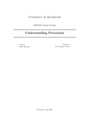
As we expect, this inertia tensor is already diagonalized because the 3-axis is a principle axisof the ring.For the purpose of numerical calculations, we will assign values to each of these parameters.A typical bicycle wheel has a radius of approximately 0.3m and weighs around 13lbs (6 kg). Wewill consider a short 0.02m axle that exaggerates the motion we are examining.3Solving the Bicycle Wheel Gyroscope with LagrangianMechanicsFigure 4: Euler angles. Image Credit: Modified from Lionel Brits [1]In order to apply Lagrangian mechanics to the problem of the gyroscope it is easiest to expressthe gyroscope’s position in terms of Euler angles. If we chose the conventions shown in figure 4,then the precessional velocity of the gyroscope will be φ̇, the nutation velocity will be θ̇, and theangular velocity of the spinning wheel itself will be ψ̇.In order to write the Lagrangian, we must first find expressions for the kinetic and potentialenergy of the gyroscope. The kinetic energy can be found by projecting the angular velocities ofthe gyroscope onto the body fixed axes:ω1 φ̇ sin θ sin ψ θ̇ cos ψ(1)ω2 φ̇ sin θ cos ψ θ̇ sin ψ(2)ω3 φ̇ cos θ ψ̇(3)Since the I1 I2 as calculated on the previous page, we can then easily write out the kineticenergy:T 111I1 ω12 I2 ω22 I3 ω3222211I1 (φ̇2 sin2 θ θ̇2 ) I3 (φ̇ cos θ ψ̇)222(4)(5)The potential energy is simply gravity:U mgs cos θ3(6)
Finally the total Lagrangian is just T U :L 11I1 (φ̇2 sin2 θ θ̇2 ) I3 (φ̇ cos θ ψ̇)2 mgs cos θ22(7)The normal process of applying Lagrange’s equation of motion to this Lagrangian by handwould be incredibly tedious. However, we can immediately see from equation 7 that both φ andψ are cyclic variables: Lp φ 0(8) φp ψ L 0 ψ(9)Which implies that both angular momentums are constant:pφ L (I1 sin2 θ I3 cos2 θ)φ̇ I3 ψ̇ cos θ constant φ̇(10) L I3 (φ̇ cos θ ψ̇) constant ψ̇(11)pψ By combining these two constants, we can thus derive an expression for the precession velocity [8]:φ̇ (pφ pψ cos θ) cos θI1 sin2 θ(12)However, at this point we reach an impasse. Fully solving these equations of motion by handwould be very difficult and extremely messy. Instead, we will use Mathematica’s differentialequation solver to numerically solve Lagrange’s equations of motion [7]. These calculations yieldthe following results for our Figure 5: Solutions to Lagrange’s Equations of MotionThe solutions in Figure 5 hint at the behavior of the gyroscope: ψ is a line (the angular velocityof the wheel remains constant) and θ oscillates back and forth above π2 . φ, the precession angle,increases, but its velocity is not constant: as the gyroscope nutates back and forth, φ (which, asseen in equation 12, is dependent on θ), φ̇ changes.4
4Explaining PrecessionWe are now in a position to illustrate an intuitive explanation of precession. Imagine that thebicycle wheel gyroscope is set spinning and held horizontally (θ π2 ). The angular momentum ofthe wheel is along the body-fixed 3 axis and thus can be attributed entirely to the rotation of thewheel about that axis.Figure 6: An angular momentum component in the z direction emerges as the gyroscope tipsdownwardWhen we let go of the wheel, it begins to fall under the force of gravity. However, whilethe angular momentum of the wheel about the body-fixed 3 axis is now pointing down below π2 2(figure 6). The conservation of angular momentum requires that the total angular momentumremain constant. Thus, a new component of angular momentum (Lφ in figure 6) must emergeso that the vector sum of Lpresent and Lφ remains constant. This new component of angularmomentum creates a rotation about the z-axis. However, rotation about the z axis is exactly thephenomenon of precession! This new component of angular momentum is the angular momentumof the precessional motion.Since angular momentum is directly proportional to angular velocity, it is now obvious thatthe precessional velocity φ̇ (equation 12) must depend on θ. This relationship can be illustratedclearly by graphing φ̇ and θ verses time (figure 7). As the gyroscope nutates, its precessionalvelocity changes to conserve the total angular momentum.Π2Φ'HtLΠ4ΘHtL0.51.1.5tFigure 7: An angular momentum component in the z direction emerges as the gyroscope tipsdownwardThis explanation of the motion shown in figure 7 makes sense until the direction of the nutationvelocity changes. However, when the wheel suddenly begins to move upward, against the force2 Remember that θ is measured from the positive z axis, so the larger θ gets, the farther the gyroscope dips belowthe horizontal.5
of gravity, our argument based on the conservation of angular momentum seems at a loss. Thismotion can be explained by looking more closely at the path followed by an individual point onthe wheel.To follow a single point on the wheel throughout its rotation we will choose a point on thewheel defined by a position vector in the body fixed frame and then transform that point into thelaboratory frame using the fact that: x, y, z λ 1 · 1, 2, 3 (13)Where λ is the Euler angle rotation matrix from the space fixed frame to the body fixed frame.Using Mathematica, we can then compute a time dependent rotation matrix λ 1 that will transform between the body fixed and lab reference frames [3]: λ 1 cos φ(t) cos ψ(t) sin φ(t) cos θ(t) sin ψ(t) cos φ(t) sin ψ(t) sin φ(t) cos θ(t) cos ψ(t)sin φ(t) sin θ(t) sin φ(t) cos ψ(t) cos φ(t) cos θ(t) sin ψ(t) sin φ(t) sin ψ(t) cos φ(t) cos θ(t) cos ψ(t) cos φ(t) sin θ(t) sin θ(t) sin ψ(t)sin θ(t) cos ψ(t)cos θ(t)We will chose a point on the whee defined by the position vector 0, R, s . Plugging λ 1into equation 13 gives a vector function P (t) that describes the motion of a point beginning at thetop of the wheel. Applying the same transformation matrix to the position vector 0, R, s gives us a similar vector function Q(t) that describes a point beginning at the bottom of the wheel.Graphing both P (t) (blue) and Q(t) (red) in the x-y plane reveals an interesting motion:y0.4y0.4x0.4 -0.4-0.4-0.4y0.4x0.4 -0.4-0.4(a) t 0.1 s. P going down, Q (b) t 0.5 s. P at the bottom,going upQ at the topx0.4-0.4(c) t 0.8 s. P going up, Qgoing downFigure 8: Trajectories of two points on the wheel. Point P (blue) begins on the top of the wheel,while point Q (red) starts at the bottom.Both points start together in the x-y plane and move apart along nearly straight lines (figure 8a). However, as point P begins to rotate around towards the bottom of the wheel, it is pushedout. Likewise, as point Q rotates up towards the top of the wheel, it is pulled in (figure 8b). Thismotion continues as the wheel comes around again: as P comes back around to the top of thewheel again in figure 8c it is pulled in, while point Q is pushed out.The motion of precession is providing a fictitious force that changes the direction of motionof these points.These forces are opposite in direction and thus do not apply a force to the centerof mass. However, they do create a torque about the center of the wheel (figure 9), opposing theforce of gravity! It is this fictitious force that keeps the gyroscope upright.6
Figure 9: The forces required to alter the trajectories of the points on the wheel exert a torqueabout the axis, supporting it against the torque of gravity5Friction and Stable PrecessionWhile precession is immediately visible when looking at an actual bicycle wheel gyroscope, nutation is much more difficult to observe. This can easily be explained by considering the frictionalforces acting at the pivot of the wheel. It is reasonable to assume these forces are approximatelyconstant, changing sign to oppose the movement of the gyroscope. However, since θ̇ is generallymuch greater than φ̇, the nutation of the gyroscope is slowed much more rapidly by frictionalforces than the precession. Over a short time the nutation motion will dampen out, leaving thegyroscope to stably precess with a fixed θ π/2.In order to quantitatively investigate this progression we can include a generalized constantfrictional force to Lagrange’s equations of motion. Frictional forces are oriented opposite to thevelocity of the particle, so we will model each force as an arbitrary constant multiplied by thevelocity unit vector in each direction:d L Lφ̇ˆ F φ̇ Fdt φ̇ φ φ̇ (14)d L Lθ̇ˆ F θ̇ F dt θ̇ θ θ̇ (15)ψ̇d L Lˆ F ψ̇ Fdt ψ̇ ψ ψ̇ (16)Where L is still given by equation 7. Again we can solve this system numerically using Mathematica. The decay to stable precession is most easily observed by considering a graph of θ(t) vs.φ(t). When F 0 we observe that this curve takes the shape of a cycloid:ΘHtL1.8Π2Figure 10: The point of the gyroscope traces out a cycloid as it precesses7
However, when we introduce a frictional force, this cycloid pattern decays:ΘHtL1.8Π2Figure 11: F -0.5; t 0 to t 3.5ΘHtL1.8Π2Figure 12: F -0.5; t 3.5 to t 6.5The gyroscope eventually settles at a constant θ. Since it continues to precess around we shouldexpect (by our arguments in the previous section) that it settles at an angle θ π/2, which isindeed the case (here θ 1.8).6ConclusionDespite its complexity, the bicycle wheel gyroscope is a rightfully iconic physics demonstration.However, to avoid confusion, it is important that some effort be made to make gyroscopic motionintuitively acceptable to students. Many intuitively satisfying models of this motion exist [2][4][5].The use of tools such as Lagrangian mechanics and numerical differential equation analysis allowsus to more effectively communicate these explanations.8
References[1] Lionel Brits. Eulerangles.svg. url: [2] Eugene Butikov. Precession and nutation of a gyroscope. European Journal of Physics,(27):1071–1081, 2006.[3] Douglas Cline. Class notes.[4] Richard Feynman. The Feynman Lectures on Physics Volume 1. Addison Wesley, 1964.[5] Svilen Kostov and Daniel Hammer. It has to go down a little, in order to go around- following Feynman on the gyroscope. url: http://arxiv.org/abs/1007.5288. arXiv:1007.5288v1[physics.pop-ph].[6] Thang V. Nguyen. motion.jpeg. url: anics/Mu TopsGyroscopes/Mu-06/Mu-06.html.[7] Superfly Physics. Gyroscopic precession. url: pic-precession.[8] Stephen T. Thorton and Jerry B. Marion. Classical Dynamics of Particles and Systems. BrooksCole, 5th edition.9
tion of classical mechanics provides the tools for a more explanatory analysis of this phe-nomenon. These techniques allow us to nd equations of motion for the gyroscope and, with the aid of computer simulations, gain a better intuitive understanding of how the gyroscope accom-plishes its seemingly impossible balancing act.