Transcription
HYDROLOGICAL PROCESSESAND MODEL REPRESENTATION:IMPACT OF SOFT DATA ON CALIBRATIONJ. G. Arnold, M. A. Youssef, H. Yen, M. J. White, A. Y. Sheshukov,A. M. Sadeghi, D. N. Moriasi, J. L. Steiner, D. M. Amatya,R. W. Skaggs, E. B. Haney, J. Jeong, M. Arabi, P. H. GowdaABSTRACT. Hydrologic and water quality models are increasingly used to determine the environmental impacts of climatevariability and land management. Due to differing model objectives and differences in monitored data, there are currentlyno universally accepted procedures for model calibration and validation in the literature. In an effort to develop acceptedmodel calibration and validation procedures or guidelines, a special collection of 22 research articles that present anddiscuss calibration strategies for 25 hydrologic and water quality models was previously assembled. The models vary inscale temporally as well as spatially from point source to the watershed level. One suggestion for future work was to synthesize relevant information from this special collection and to identify significant calibration and validation topics. Theobjective of this article is to discuss the importance of accurate representation of model processes and its impact on calibration and scenario analysis using the information from these 22 research articles and other relevant literature. Modelsare divided into three categories: (1) flow, heat, and solute transport, (2) field scale, and (3) watershed scale. Processessimulated by models in each category are reviewed and discussed. In this article, model case studies are used to illustratesituations in which a model can show excellent statistical agreement with measured stream gauge data, while misrepresented processes (water balance, nutrient balance, sediment source/sinks) within a field or watershed can cause errorswhen running management scenarios. These errors may be amplified at the watershed scale where additional sources andtransport processes are simulated. To account for processes in calibration, a diagnostic approach is recommended usingboth hard and soft data. The diagnostic approach looks atsignature patterns of behavior of model outputs to determine which processes, and thus parameters representingSubmitted for review in April 2014 as manuscript number SW 10726;them, need further adjustment during calibration. Thisapproved for publication by the Soil & Water Division of ASABE inovercomes the weaknesses of traditional regression-basedOctober 2014.calibration by discriminating between multiple processesMention of company or trade names is for description only and doeswithin a budget. Hard data are defined as long-term,not imply endorsement by the USDA. The USDA is an equal opportunityprovider and employer.measured time series, typically at a point within a waterThe authors are Jeffrey G. Arnold, ASABE Fellow, Agriculturalshed. Soft data are defined as information on individualEngineer, USDA-ARS Grassland Soil and Water Research Laboratory,processes within a budget that may not be directly measTemple, Texas; Mohamed A. Youssef, ASABE Member, Associateured within the study area, may be just an average annualProfessor, Department of Biological and Agricultural Engineering, NorthCarolina State University, Raleigh, North Carolina; Haw Yen, Postestimate, and may entail considerable uncertainty. TheDoctoral Research Associate, Texas AgriLife Research, Temple, Texas;advantage of developing soft data sets for calibration isMichael J. White, Agricultural Engineer, USDA-ARS Grassland Soil andthat they require a basic understanding of processes (waWater Research Laboratory, Temple, Texas; Aleksey Y. Sheshukov,ter, sediment, nutrient, and carbon budgets) within the spaASABE Member, Assistant Professor, Department of Biological andtial area being modeled and constrain the calibration.Agricultural Engineering, Kansas State University, Manhattan, Kansas;Ali M. Sadeghi, Soil Scientist, USDA-ARS Hydrology and RemoteKeywords: Calibration, Field-scale models, Point models,Sensing Laboratory, Beltsville, Maryland; Daniel N. Moriasi, ASABEValidation, Watershed models.Member, Research Hydrologist, and Jean L. Steiner, Supervisory SoilScientist, USDA-ARS Grazinglands Research Laboratory, El Reno,Oklahoma; Devendra M. Amatya, ASABE Member, ResearchHydrologist, USDA Forest Service, Cordesville, South Carolina; R.Wayne Skaggs, ASABE Fellow, W. N. Reynolds and DistinguishedUniversity Professor, Department of Biological and AgriculturalEngineering, North Carolina State University, Raleigh, North Carolina;Elizabeth B. Haney, Graduate Research Assistant, and Jaehak Jeong,ASABE Member, Assistant Professor, Texas AgriLife Research, Temple,Texas; Mazdak Arabi, Assistant Professor, Department of Civil andEnvironmental Engineering, Colorado State University, Ft. Collins,Colorado; Prasanna H. Gowda, ASABE Member, Research AgriculturalEngineer, USDA-ARS Conservation and Production Research Laboratory,Bushland, Texas. Corresponding author: Jeffrey Arnold, USDA-ARSGSWRL, 808 East Blackland Road, Temple, TX; phone: 254-770-6508; email: jeff.arnold@ars.usda.gov.Water quality and hydrologic models are commonly used to assess the environmental impacts of land management and policy decisions. Models are increasingly being appliedto large varied agricultural landscapes to address contemporary water resource issues in the context of climatechange and sea level rise (Jayakrishnan et al., 2005). Moriasi et al. (2012) summarized the calibration approaches of25 models in a special collection of 22 articles, each focus-Transactions of the ASABEVol. 58(6): 1637-16602015 American Society of Agricultural and Biological Engineers ISSN 2151-0032 DOI 10.13031/trans.58.107261637
ing on the individual model calibration and validation strategies. These models vary in scope from field-scale modelsthat focus on flow, heat, and solute transport to large-scalewatershed models that incorporate complex processes overspatially diverse subwatersheds. Regardless of scale, modelaccuracy is improved through calibration, and model uncertainty (thus utility) is evaluated via validation. Calibrationand validation are important factors in the development ofmeaningful model predictions of potential future land useor climate effects. There are no universal standards for thecalibration and validation of models in the current literature, as the procedure is generally dependent upon the processes in play at each model scale. Basic model processesinclude hydrology (water budget), erosion and sedimentation, plant growth, nutrient and carbon cycling, and contaminant fate and transport. Model processes, in varyingdegrees, are interconnected and impacted by land management, topography, climate, and scale. Point-scale modelsare used primarily to simulate physical and biological processes such as water and heat flow and reactive solutetransport through a soil column and may be in finer timescales of less than an hour. At the field scale, the waterbalance processes include many variables that are interdependent with other processes, such as plant growth, soilproperties, and weather. Nutrient cycling processes arecomplex and may vary greatly depending upon soil conditions even at the field scale. The carbon cycle appears simple at first glance; however, individual components, such asphotosynthesis and soil carbon dynamics, are complex tosimulate using a model. For example, photosynthesis isvegetation dependent and is influenced by resource (light,water, and nutrients) availability and environmental conditions. Soil carbon dynamics are influenced by the amountand biochemical composition of the soil organic matter, thequantity and quality (determined by C:N ratio and lignincontent) of organic matter input (e.g., plant residue, animalmanure, litter fall, root turnover) to the soil, and environmental factors (soil water and temperature) affecting biological activity. All of these factors influence the rate ofsoil organic carbon decomposition and the interaction between the mineral and organic forms of nitrogen and phosphorus (Youssef et al., 2005).Model calibration techniques range from iterative manual methods to the use of fully automated calibration software. Field-scale models often simulate the main hydrological and biogeochemical processes, including infiltrationand soil water distribution in the vadose zone, evapotranspiration, subsurface drainage, surface runoff, soil erosion,sediment transport, pesticide and nutrients dynamics, soilcarbon cycling, and plant growth, for one or more plots orfields. Field-scale models are calibrated using manual orautomated methods; both methods focus on hydrologic,chemical, or biologic parameters. Large-scale watershedmodels simulate complex hydrologic processes on a watershed or basin scale, in addition to the above processes ineach plot or field. These processes include ditch/channel/riparian and reservoir processes, erosion and sedimentmovement and deposition, stream transport of nutrients,nutrient or pesticide degradation and transformation, water/air interactions, complex soil/plant/climate interactions,1638algae and aquatic plants, and cycling in floodplains, estuaries, wetlands, and large hydraulic structures. Processes considered and calibration techniques used by each of the 25models are described in the special collection (Moriasi etal., 2012).This article describes the importance of realisticallysimulating all critical processes in the hydrological balancefor calibration and validation of small- and large-scalemodels. For example, if surface runoff is overestimated, itis likely that evapotranspiration (ET) and/or subsurface andtile flow are underestimated, resulting in overestimation ofsediment yields and underestimation of subsurface nitrateand other soluble contaminant yields. This will cause further error when parameterizing variables related to sediment and nutrient transport and result in unrealistic policyrecommendations when running scenarios that target erosion and fertilizer management. Problems are even morecompounded at the watershed scale when multiple fields orsubbasins are simulated and output is routed through channels, flood plains, and reservoirs. Thus, it is important toreasonably simulate nutrient and sediment sources andsinks within a watershed in addition to their loads at agauging station (outlet). If upland erosion is overpredicted,channel erosion must be underpredicted to match measuredgauge loads. The management practices designed to reduceerosion from the landscape may then show significant impact on total sediment yields, while in reality the practiceswould have little impact at the basin outlet. It is also important at the watershed scale to accurately simulate propersource load allocations. For example, excellent calibrationstatistics can be obtained at a stream gauge outlet eventhough point sources are underestimated and the loads fromagricultural lands are overestimated. This could result inpolicy scenarios that overestimate the impact of conservation or best management practices (BMPs) on agriculturaland forested lands. For most models, little guidance is provided for considering process representation in the calibration and validation procedures.The objectives of this article are to: (1) synthesize processes considered and calibration techniques used to account for processes within a field or watershed for themodels in the special collection (Moriasi et al., 2012),(2) summarize other relevant literature related to processrepresentation and calibration, (3) demonstrate the importance of proper process representation utilizing soft dataand its impact on calibration/validation scenario analysisusing case studies, and (4) provide recommendations forcalibration/validation.SYNTHESIS OF PROCESSES SIMULATEDBY MODELS IN SPECIAL COLLECTIONThe 25 hydrologic and water quality models in the special collection of calibration and validation concepts summarized by Moriasi et al. (2012) are categorized as:(1) flow, heat, and solute transport models, (2) field-scalemodels, and (3) watershed-scale models in order to facilitate discussion and compare concepts. Different approacheswere taken for describing the processes in each categoryTRANSACTIONS OF THE ASABE
due to general differences in the processes. For flow, heat,and solute transport models, the equations and solutiontechniques are similar in each model, so we described thegeneral processes and then noted any models that differedfrom the general approach. Since all field-scale modelsrepresented the same basic processes of hydrology, soilerosion and sediment transport, vegetation, carbon, nitrogen and phosphorus, and pesticides, we divided the discussion by process and then described how each model simulated that process. Since watershed-scale models generallyrepresent processes of more spatial and temporal complexity, the processes and calibration concepts of each modelwere summarized individually. Not only do watershed-scale models consider additional processes, they often employ significantly different levels of complexity. Table 1shows the scale or dimension of each model, the processesthat are represented, and typical calibration techniques.FLOW, HEAT, AND SOLUTE TRANSPORT MODELSPoint-scale models are usually suited for modeling processes that are mostly one-dimensional, at soil profile orhorizon column, and represent a single footprint at the surface. Models considered include SHAW, COUPMODEL,SWIM3, MACRO, VS2DI, HYDRUS, STANMOD, andTOUGH (table 1). These models are normally used toquantify the basic physical or chemical processes that occurTable 1. Scale and calibration processes considered by 25 models in the special collection of 22 articles (Moriasi et al., 2012).ModelReferenceScale/DimensionModel ProcessesTypical Calibration TechniquesFlow, heat, and solute transport modelsSHAWFlerchinger1-DSoil water, heat, and solute concen- Sensitivity analysis, manual or automated. Stepet al., 2012trationswise, trial and error, optimization algorithmCOUPMODELJansson,1-DHydrology, erosion, pesticides,Manual and automated, stepwise systematic, use2012sediments, nutrients, plant growth of double mass plot techniqueSWIM3Huth et al.,1-DWater and solute transportManual, water balance2012MACROJarvis and1-DMacropore flow, pesticidesForward, sequential and iterative procedureLarsbo, 2012VS2DIHealy and2-DWater, heat, and solute transportManual, parameter estimation programsEssaid, 2012HYDRUSŠimůnek et al.,1, 2, or 3-DWater, heat, and solute transport,Gradient-based local optimization or automated2012carbon dioxide fluxSTANMODvan Genuchten1, 2, or 3-DSolute transport in soils andWeighted nonlinear least square methodet al., 2012groundwaterMT3DMSZheng et al.,1, 2, or 3-DMultispecies solute transportManual and automated, variance-covariance ma2012trixTOUGHFinsterle et al.,1, 2, or 3-DMultiphase, multicomponent fluid Weighted least squares objective function2012flows in porous and fracture geologic mediaField-scale modelsDRAINMODSkaggs et al.,FieldHydrology, carbon and nitrogenManual, stepwise, iterative2012cycles, plant growthADAPTGowda et al.,FieldHydrology, erosion, nutrients,Partition flows, annual water and nutrient balanc2012pesticides, subsurface tile drainage esCREAMS/GLEAMSKnisel andFieldEdge of field sediment, nutrientManual, stepwise: hydrology, sediment, nutriDouglas-Mankin,and pesticide lossesents/pesticides2012RZWQM2Ma et al.,PointHydrology, plant growth, nutrients, Manualpesticides2012EPICWang et al.,FieldHydrology, carbon and nitrogenManual and automated, multi-site data2012cycles, plant growthWEPP HillslopeFlanaganHillslopeHydrology, soil erosion across theet al., 2012landscapeStepwise: bioclimate, vegetation, soil and fieldDAISYHansen et al.,PointHydrology, carbon cycle, energy2012balance, nitrogen, crop production, management parameterspesticidesWatershed-scale modelsAPEXWang et al.,Small watershed/ Hydrology and plant growthManual and automated, multi-site data2012whole farmWEPP WatershedFlanaganSmall watershed Hydrology, soil erosionStepwise procedure: hydrology, erosionet al., 2012SWATArnold et al.,Watershed to Hydrology, plant growth, sediManual and automated, multi-site data2012river basinment, nutrients, pesticidesHSPFDuda et al.,Watershed to Hydrology, snowmelt, pollutantIterative procedure of parameter evaluation and2012river basinloadings, erosion, fate andrefinementtransportWAMBottcher et al.,Watershed to Hydrology, sediments, nutrientsManual and automated, multi-site data2012river basinKINEROSGoodrichWatershedStreamflow and sedimentSimple manual to complex automatedet al., 2012MIKE-SHEJaber andWatershed to Surface and subsurface water dyManual and automated(DAISY coupling)Shukla, 2012river basinnamics, evapotranspiration, flow,water quality58(6): 1637-16601639
during the transport of water, exchange or transfer of heat,and/or movement of various nutrients, pollutants, pathogens, and carbon through the unsaturated zone (or vadosezone) in a soil column. The fate and transport processesoccurring near the soil surface profiles are mostly dependent on soil properties but are also affected by the earthatmosphere surface and the bottom of the column subsurface boundary conditions. These models have a varyingdegree of complexity and can be multidimensional. Analytical solutions can be sought for one-dimensional simplifiedformulations, especially under steady-state conditions,whereas a numerical approach is developed for multivariable non-linear physical processes. Commonly used,physically based approaches to solve processes in the soilprofile are discussed in the following sections.Water Flow EquationAll point-scale models consider water movement in thesoil profile that generally occurs under two conditions, saturated or unsaturated. The saturated condition, however, isa special case of the unsaturated condition and occurs whenthe soil moisture content is at a maximum level for a particular soil type. Darcy’s law (Darcy, 1856) was the firstmathematical description of water movement in soil thatshowed the proportionality of the flux of water to the hydraulic gradient: q k H(1) where q is the soil water flux, k is the proportionality factor, which is known as the hydraulic conductivity, and His the gradient of the hydraulic head H in the multidimensional space.Equation 1 is commonly used to evaluate a situation inwhich a steady-state flow or near steady-state prevails, thatis, the flux remains constant at any point along the conducting water flow system. In the actual field conditions, however, most soil water transport processes occur under transient-state conditions, where the magnitude and the direction of the flux and hydraulic gradient vary with time.Therefore, considering the law of conservation of mass, inthe multidimensional system, the relationship betweenchange in soil moisture content (θ) and flux (q) or H can beexpressed as: θ θ q or k H t t(2)Equation 2, called the Richards equation (Richards,1931), must be supplemented by the soil constituent relationships k(θ) and H(θ) that can be found from hydraulicexperiments on the soil column. The Richards equation iswidely used in point-scale models and is considered a cornerstone of water flow formulations that represent mostlythe movement of water in unsaturated soils. It is a nonlinear partial differential equation and has a limited numberof closed-form analytical solutions that were developed forspecial cases of homogeneous soils with simplified functional forms of k(θ) and H(θ), and certain initial andboundary conditions (Philip, 1969, 1972, 1992; Wooding,1968). Most of these solutions consider infiltration applica-1640tions and assume constant water content or flux values forsteady-state water flow conditions. Šimůnek et al. (1999)reported that a large number of analytical models for one-,two-, and three-dimensional solute transport problems wererecently incorporated into the comprehensive softwarepackage STANMOD (van Genuchten et al., 2012).Several numerical methods based on finite difference,finite volumes, or finite element approximations have beendeveloped to solve the water flow equation in unsaturatedporous media and utilize the H-based form, θ-based form,or H-θ mixed form of equation 2. In most numericalschemes, the storage term is linearized using the NewtonRaphson or Picard methods, and equation 2 is solved iteratively. Such an approach is implemented in HYDRUS(Šimůnek et al., 1998), SWAP (van Dam et al., 1997), andMODFLOW-2000 (Thoms et al., 2006).The SHAW model (Flerchinger and Saxton, 1989), forexample, is one of the point-scale models that uses a modified form of the Richards equation and simulates heat andwater movement through a plant residue-soil system. Thisone-dimensional model considers a profile that extendsfrom the vegetation canopy to a specified depth within thesoil profile. Preferential or macropore flow represents rapidflow of water and chemicals through porous media such assoil profiles and has recently attracted the attention of scientists and modelers working in the environmental field.Incorporation of this rapid movement of pollutants from theupper soil profile into lower behavior has created a multitude of difficulties in modeling vadose zone transport. Oneof the approaches used in dual-porosity models considersthat main flow occurs in preferential flow paths while wateris immobile in the soil matrix. For example, the modelMACRO (Jarvis and Larsbo, 2012) uses a capacitance approach to calculate macropore flow, while the Richardsequation is used to model micropore flow in the soil matrix.The more sophisticated approach is sought to describe theinfiltrating flow under very dry conditions where flowbreaks into fingers, but the Richards equation has proved tobe unconditionally stable (Egorov et al., 2003). This approach looks at the flow process being non-equilibrium andassumes a kinetic relationship between water content andmatrix head (Nieber et al., 2005; Chapwanya and Stockie,2010).Reactive Contaminant TransportMany models, such as SHAW, STANMOD, VS2DI(Healy and Essaid, 2012), and SWIM3 (Huth et al., 2012),can simulate transport of reactive contaminants simultaneously with water flow. In these models, after water fluxes q are quantified in equations 1 and 2, a physically basedmodel of reactive contaminant transport can be described asan advective-dispersive transport problem with the diffusive flux considered based on Fick’s law (Fick, 1855) andsolute subject to sorption and degradation on the soil parti cles. The flux qc explains the mass of solute (C) or anyother pollutants diffusing across a unit cross-sectional areaper unit time as: qc D C qC(3)TRANSACTIONS OF THE ASABE
where D is the solute dispersion coefficient and can be afunction of θ. Thus, by substituting equation 3 into the general expression of the flux of the solute change in the vertical direction per unit volume and unit time, a flow equationwill result that encompasses both dispersion and mass flowcomponents for solute transport in the soil profile: ( θ C Cs ) t D C ( qC )(4)where Cs is the concentration of contaminant in the sorbedphase and subject to the sorption law. The solution of equation 4 requires both initial and boundary conditions.Heat TransferThe heat transfer in the soil column is usually modeledby the convection-conduction equation:c θ T L s λ T cw ( qT ) t t(5)where T is the temperature, c is the heat capacity, λ is thethermal conductivity, and L is the latent heat of evaporationor freezing. The second term in the left side of equation 5accounts for the heat released during water phase change(freezing or evaporation) and was included in models suchas SHAW.Other Transport ProcessesMany existing models, such as COUPMODEL, SWIM3,MACRO, VS2DI, HYDRUS, STANMOD, MT3DMS(Zheng et al., 2012), and TOUGH (Finsterle et al., 2012),can also model a variety of other physical and chemicalprocesses: nutrient and carbon cycle, gas diffusion, icebuildup, soil freezing and melting, colloid detachment andmovement, transport of charged particles, pesticidetransport, etc. For example, the PRZM model (Carsel et al.,1985) was originally developed to assess pesticide fate andtransport within the crop’s root zone but was recently coupled with the VADOFT model (Mullins et al., 1993) tosolve the Richards equation in the vadose zone. Despitemajor recent modifications, the model still lacks amacropore and preferential flow component (Sadeghi et al.,1995).Surface Boundary ConditionsMost of the point-scale models (DAISY, SHAW,SWAP, HYDRUS, and COUP, among others) are subjectto complex non-linear upper boundary conditions at theearth-atmosphere surface. These conditions evaluate waterand energy budgets and provide values for surface flow,infiltration rates, and water vapor and heat fluxes. Twomain conditions that work at various temporal scales andthat point-scale models account for are the water budgetand energy budget conditions, which can generally be written as:( P E ) A Qi Qo dWdt(6)R L E H G(7)where P is the rate of precipitation, E is the rate of evapora-58(6): 1637-1660tion, A is the footprint surface area, Qi and Qo are the surface inflow and outflow rates, W is the water volume storedat the surface footprint, R is the net incoming radiation flux,and H and G are the specific fluxes of sensible and conductive heat. The equations at the surface boundary (eqs. 6 and7) link inputs taken from climate models (P and R) with thevariables dependent on processes inside the column, landcover, input from adjacent columns, etc. Most onedimensional point-scale models simulate flow and transportin the column only vertically and assume that excess waterat the surface boundary is removed by surface runoff. Interconnectivity of flow between vertical columns is considered in multi-dimensional point-scale models by modelingtwo- or three-dimensional processes in the column (eqs. 1through 5) as well as overland processes at the surface.More advanced linkage of surface processes with inputsfrom soil is included in hillslope or field-scale models.FIELD-SCALE MODELSThe field-scale models in the special issue(CREAMS/GLEAMS, DRAINMOD, ADAPT, RZWQM,EPIC, WEPP Hillslope, and DAISY) were developed tosimulate the physical, chemical, and biological processesoccurring in the soil-water-plant system and have been usedto simulate the effects of management practices on agricultural production and soil and water resources with the goalof increasing productivity, reducing cost, and enhancingsustainability. Simulated agricultural management practicesinclude crop rotations, fertilizer management practices,tillage and plant residue management practices, land application of animal manure, irrigation, and drainage watermanagement. These models usually simulate the water balance (fig. 1), plant growth, nutrient cycling in soil (fig. 2),carbon dynamics (fig. 3), pesticide dynamics, and agriculture land management. Depending on the model, predictions can be a subset of crop/biomass yield, edge-of-fieldsurface, subsurface and tile flow, sediment nitrogen, phosphorus, and pesticide losses, and nitrogen and soluble pesticide losses via surface runoff and leaching.Over the years, field-scale models have been expandedand enhanced. GLEAMS was developed by improvingCREAMS to better represent soil layers, crop rotations, andchemical transport. EPIC was also developed by improvingGLEAMS to better represent cropping systems and management while accounting for the impact of erosion on cropproductivity (Williams et al., 2008; Wang et al., 2012).ADAPT was developed as a water management model forhigh water table soils by incorporating DRAINMOD-basedroutines for tile drainage and water table simulation intoGLEAMS (Gowda et al., 2012). RZWQM development inthe mid-1980s and early 1990s was based on existing models including CREAMS, GLEAMS, Opus, and PRZM. Later, the model was further improved by incorporating theSHAW model for conducting full energy balance at the soilsurface, DRAINMOD-based routines for tile drainage, andDSSAT crop modules for simulating crop growth and yield(Ma et al., 2012). The current version of RZWQM is considered an agricultural system model that simulates cropyield, water and nitrogen balances, and pesticide fate asinfluenced by management practices, soil properties, and1641
Figure 1. Hydrologic processes in the water balance (adapted from Arnold et al., 2000).Figure 2. Processes in the nitrogen cycle.climatic conditions. DRAINMOD was developed in the late1970s as a hydrological model for simulating the performance of agricultural drainage and related water management systems. Over the years, the model has been expanded and enhanced to become a system model for simulatinghydrology, soil carbon and nitrogen dynamics, and vegetation growth for agricultural and forest ecosystems on poorly or artificially drained shallow water table soils (Skaggs1642et al., 2012). The WEPP Hillslope model was developed inthe early 1980s to replace the USLE (Flanagan et al.,2012). Original water balance, plant growth, and nutrientcomponents in WEPP were modified from the EPIC model.The term “field” as a spatial scale could be defined as aspatial unit with homogeneous characteristics, includingweather, soil, topography, cropping system, and manage-TRANSACTIONS OF THE ASABE
The field-scale models reviewed in this article can becategorized as process-based or more precisely as “hybrid”models. In hybrid models, some processes are empiricallyrepresented in the model structure in order to reduce inputrequirement and reduce uncertainty in model predictionswhile maintaining the key advantages of process-basedmodels. The models differ in their level of detail in simulating different physical, chemical, and biological processesoccurring in the soil-water-plant system.HydrologyFigure 3. The carbon cycle (courtesy of th
techniques are similar in each model, so we described the general processes and then noted any models that differed from the general approach. Since all field-scale models represented the same basic processes of hydrology, soil erosion and sediment transport, vegetation, carbon, nitro-gen and phosphorus, and pesticides, we divided the discus-