Transcription
Recent Advances in EmbeddedModel Predictive ControlAlberto Bemporadhttp://cse.lab.imtlucca.it/ bemporadICSTCC’18 - Sinaia, Romania - 11/10/2018
Outline Model Predictive Control (MPC) (in a nutshell) Recent advances in embedded quadratic programming (QP) solvers Data-driven design of embedded MPC controllers Embedded MPC in industry2/38
Model Predictive Control (MPC)optimizationprediction modelalgorithmmodel-based optimizerprocess1mins.t.r(t)2 x0Ax Qx c lifiedlikelyUse a dynamical model of the process to predict its futureevolution and choose-------------------the “best” control actiona good3/38
Model Predictive Control (MPC) Goal: find the best control sequence over a future horizon of N stepspastminN 1 y W (yk 2r(t)) 2u W (uk futurexk 1 f (xk , uk )yk g(xk , uk )prediction modelumin uk umaxymin yk ymaxconstraintsx0 x(t)state feedbackmanipulated inputstoptimization problempredicted outputsukk 0s.t.r(t)yk2ur (t)) 2t kt 1t 1 kt Nt N 1 At each time t:– get new measurements to update the estimate of the current state x(t)– solve the optimization problem with respect to {u0 , . . . , uN 1 }– apply only the first optimal move u(t) u 0 , discard the remaining samples4/38
MPC in industry The MPC concept for process control dates back to the 60’s(Rafal, Stevens, AiChE Journal, 1968) MPC used in the process industries since the 80’s(Qin, Badgewell, 2003) (Bauer, Craig, 2008)MPC is the standard for advanced control in the process industry Research in MPC is still very active !5/38
d 23dingy ofwith,y; ally ine re stry,govencectorsencepace,cals,dical,geowithd allf theC naech-stantial benefits in each of severalindustry sectors; adoption byma ny companies in different sectors; standard practice in industry.» High single-industry impact: Substantial benefits in one industrysector; adoption by many compa-MPC in industry, thenteranyease.org.(or discovery), we still have nothing that compares with PID! It’s alsoconcerning that the “crown jewels”of control theory appear near the bot(Samad, IEEE CS Magazine, 2017)tom of the list. However, the fact thatall the technologies had at least somepositive assessments suggests that theImpact of advanced control technologies in industryTABLE 1 A list of the survey results in order of industry impact as perceived bythe committee members.Rank and TechnologyHigh-Impact RatingsLow- or No-Impact RatingsPID control100%0%Model predictive control78%9%System identification61%9%Process data analytics61%17%Soft sensing52%22%Fault detection andidentification50%18%Decentralized and/orcoordinated control48%30%Intelligent control35%30%Discrete-event systems23%32%Nonlinear control22%35%Adaptive control17%43%Robust control13%43%Hybrid dynamical systems13%43%6/38FEBRUARY 2017« IEEE CONTROL SYSTEMS MAGAZINE17
Automotive applications of MPC(Bemporad, Bernardini, Borrelli, Cimini, Di Cairano, Esen, Giorgetti, Graf-Plessen, Hrovat, KolmanovskyLevijoki, Ripaccioli, Trimboli, Tseng, Yanakiev, . (2001-present))Ford Motor CompanyPowertrainengine control, magnetic actuators, robotized gearbox,power MGT in HEVs, cabin heat control, electrical motorsJaguarDENSO AutomotiveVehicle dynamicstraction control, active steering, semiactive suspensions,autonomous drivingFCAGeneral MotorsModel predictive control tire deflectiontire deflection 44Most automotive OEMs are looking into MPC solutions today7/38
MPC for autonomous driving Coordinate torque request and steering to achieve safe andcomfortable autonomous driving with no collisions MPC combines path planning, path tracking, and obstacleavoidance Stochastic prediction models are used to account for uncertaintyand driver’s behavior8/38
MPC of gasoline turbocharged engines Optimize engine actuators (throttle, wastegate, intake/exhaust cams) to makeengine torque track set-points, maximizing efficiency and satisfying AchievedTorqueMeasurementsQP solved in real-time on ECU(Bemporad, Bernardini, Long, Verdejo, 2018)engine operating at low pressure (66 kPa)9/38
Supervisory MPC of powertrain with CVT Coordinate engine torque request and continuously variable transmission(CVT) ratio to improve fuel economy and drivability Real-time MPC is able to take into account coupled dynamics and constraints,optimizing performance also during transientsEnginetorquerequestDesiredaxle torqueEngine ControlMPCCVTratiorequestCVT ControlUS06 Double Hill driving cycle(Bemporad, Bernardini, Livshiz, Pattipati, 2018)10/38
Aerospace applications of MPC MPC capabilities explored in new space applicationscooperating UAVspowered descent (Bemporad, Rocchi, 2011)planetary rover (Pascucci, Bennani, Bemporad, 2016) (Krenn et. al., 2012)11/38
MPC for Smart Electricity Grids(Patrinos, Trimboli, Bemporad, 2011)transmission gridcoal 1? ?photovoltaiccoal 2hydro-storage? ? ? ? ?demandnatural gas? ? ?wind farmDispatch power in smart distribution grids, trade energy on energy marketsChallenges: account for dynamics, network topology, physical constraints, andstochasticity (of renewable energy, demand, electricity prices)FP7-ICT project “E-PRICE - Price-based Control of Electrical Power Systems”(2010-2013)12/38
Embedded Linear MPC and Quadratic Programming Linear MPC requires solving a Quadratic Program (QP)minzs.t.1 ′z Qz x′ (t)F ′ z2Gz W Sx(t) z u0u1. Ax bx*1 x0 Qx c0 x constant2uN 1(Beale, 1955)A rich set of good QP algorithms is available today Which QP algorithms are suitable for implementation in embedded systems ?13/38
MPC in a production environmentKey requirements for deploying MPC in production: 0 Qx1 xb2x nmi . As.tcx01. speed (throughput)– worst-case execution time less than sampling interval– also fast on average (to free the processor to execute other tasks)2. limited memory and CPU power (e.g., 150 MHz / 50 kB)3. numerical robustness (single precision arithmetic)4. certification of worst-case execution time5. code simple enough to be validated/verified/certified(library-free C code, easy to check by production engineers)14/38
Embedded solvers in industrial production Multivariable MPC controller Sampling frequency 40 Hz ( 1 QP solved every 25 ms) Vehicle operating 1 hr/day for 360 days/year on average Controller running on 10 million vehicles 520,000,000,000,000 QP/yrand none of them should fail.15/38
Fast gradient projection(Nesterov, 1983) (Patrinos, Bemporad, 2014) Solve (dual) QP by fast gradient method1 ′z Qz x′ F ′ z2Gz W Sxminzs.t.KgL Q 1 G′Q 1 F xβk max{ k 1, 0}k 21λmax (GQ 1 G′ )wk y k βk (y k y k 1 )zk Kwk gsk y k 11kL Gz 1L (W Sx)}kk max w s , 0{while k maxiterbeta max((k-1)/(k 2),0);w y beta*(y-y0);z -(iMG*w iMc);s GL*z-bL;y0 y;% Terminationif all(s epsGL)gapL -w'*s;if gapL epsVLreturnendendy w s;k k 1;end Very simple to code Convergence rate: f (xk ) f (x ) (Necoara, Nesterov, Glineur, 2018)2L z0 z 22(k 2)2 Tight bounds on maximum number of iterations Extended to mixed-integer quadratic programming (MIQP) (Naik, Bemporad, 2017)16/38
ADMM(Gabay, Mercier, 1976) (Glowinski, Marrocco, 1975) (Douglas, Rachford, 1956) (Boyd et al., 2010) Alternating Directions Method of Multipliers for QPz k 1sk 1uk 1 (Q ρA′ A) 1 (ρA′ (uk sk ) c) min{max{Az k 1 uk , ℓ}, u} uk Axk 1 sk 1mins.t.1 ′z Qz2 c′ zℓ Az uwhile k maxiterk k 1;z -iM*(c A'*(rho*(u-s)));Az A*z;s max(min(Az u,ub),lb);u u Az-s;end(7 lines EML code)( 40 lines of C code)ρu dual vector Matrix (Q ρA′ A) must be nonsingular The factorization of matrix (Q ρA′ A) can be done at start and cached Very simple to code. Sensitive to matrix scaling (as gradient projection) Used in many applications (control, signal processing, machine learning)17/38
Regularized ADMM for quadratic programming(Banjac, Stellato, Moehle, Goulart, Bemporad, Boyd, 2017) Robust “regularized” ADMM iterations:z k 1sk 1uk 1 (Q ρAT A ϵI) 1 (c ϵzk ρAT (uk z k )) min{max{Az k 1 y k , ℓ}, u} uk Az k 1 sk 1 Works for any Q 0, A, and choice of ϵ 0 Simple to code, fast, and robust[ Only needs to factorizeQ ϵIAA′ ρ1 I Implemented in free osQP solver]oncehttp://osqp.org(Python interface: 20,000 downloads) Extended to solve mixed-integer quadratic programming problems(Stellato, Naik, Bemporad, Goulart, Boyd, 2018)18/38
QP solvers - An experimental comparison Experimental setup:– PC with MATLAB/Simulink– RS232 adapter– TMS320F28335 DSP (150 MHz)vars constr.4 168 2412 32ODYS QP0.12 ms0.44 ms1.2 msGPAD0.33 ms1.1 ms2.6 msADMM1.4 ms4 ms8.2 ms Active set (AS) methods are usually the best on small/medium problems:– excellent quality solutions within few iterations– behavior is more predictable ( less sensitive to preconditioning)– no need for advanced linear algebra libraries19/38
Can we solve QP’s using least squares ?The least squares (LS) problem is probably themost studied problem in numerical linear algebraAdrien-Marie Legendre(1752–1833)v arg min Av b 22In MATLAB: v A\b(one character !)Carl Friedrich Gauss(1777–1855) Nonnegative Least Squares (NNLS):(Lawson, Hanson, 1974)minv Av b 22s.t. v 0very simple to solve (750 chars in Embedded MATLAB)20/38
Solving QP’s via nonnegative least squares(Bemporad, 2016) Complete the squares and transform QP to least distance problem (LDP)minz1 ′2 z Qz c′ zQ L′ Ls.t. Gz gminus.t. M u du , Lz L T c An LDP can be solved by the NNLSminy12122 u (Lawson, Hanson, 1974)[M′d′][ ]0y 1s.t. y 022M GL 1d b GQ 1 c If residual 0 then QP is infeasible. Otherwise setz 1L 1 M ′ y Q 1 c1 d′ y Extended to solving mixed-integer QP’s(Bemporad, NMPC, 2015)21/38
Solving QP’s via NNLS and proximal point iterations(Bemporad, 2018) Solve QP via NNLS within proximal-point iterationszk 1 arg minzs.t.1 ′2 z Qz c′ z 2ϵ z zk 22Az bGx g Advantage: numerical robustness, as Q ϵI can be arbitrarily well conditionedsingle precision arithmetic30 vars, 100 constraints(Macbook Pro 3 GHz Intel Core i7) Extended to solve MIQP problems(Naik, Bemporad, 2018)22/38
MPC without on-line QPoptimizationprediction modelalgorithmmodel-based optimizerprocess1mins.t.r(t)2 x0Ax Qx c x0bset-pointsinputsoutputsu(t)y(t)measurements Can we implement MPC without an on-line solver ?23/38
Explicit model predictive control and multiparametric QP(Bemporad, Morari, Dua, Pistikopoulos, 2002) The multiparametric solution of a strictly convex QP is continuous andpiecewise affinez (x) arg minz 12 z ′ Qz x′ F ′ zs.t. Gz W Sx Corollary: linear MPC is continuous & piecewise affine ! z u0u1.u N 1 u 0 (x) F1 x g1. . FM x gMififH1 x K1.HM x KM New mpQP solver based on NNLS available (Bemporad, 2015)and included in MPC Toolbox since R2014b (Bemporad, Morari, Ricker, 1998-today)Is explicit MPC better than on-line QP ( implicit MPC) ?24/38
Complexity certification for active-set QP solvers Result: The number of iterations to solve the QP via a dual active-set method isa piecewise constant function of the parameter x(Cimini, Bemporad, 2017)We can exactly quantify howmany iterations (flops) the QPsolver takes in the worst-case ! Examples (from MPC Toolbox):Explicit MPCmax flopsmax memory (kB)Implicit MPCmax flopssqrtmax memory (kB)inverted pendulumDC motornonlinear demoAFTI 72078073316 QP certification algorithm currently used in production25/38Model predictive control toolset1/8
Certification of KR solver The KR algorithm is a very simple and effective solver for box-constrained QP.All violated/active constraints form the new active set at the next iteration(Kunisch, Rendl, 2003) (Hungerländer, Rendl, 2015) Assumptions for convergence are quite conservative, and indeed KR can cycleWe can exactly map how many iterations KR takes to converge (or cycle)(Cimini, Bemporad, 2019)# of iterations123456Example 1Example 2Example 3Explicit MPCmax flopsmax memory [kB]3243.97183015.9540189.69Dual active-setmax flops sqrtmax memory [kB]580 58.211922 138.633622 248.90KR algorithmmax flopsmax memory [kB]4893.1914543.3929613.51regions where KR fails2θ210 1 201234θ1Figure 2. Complexity certification of the KR algorithm forthe toy QP problem (19). The black regions represent subsetsof the parameter space for which the KR algorithm cycles.26/38
Data-driven MPC
MPC and Machine Learning Model predictive control requires a model of the process Models are usually obtained from data (parameter estimation or black-boxmodeling)In industrial MPC most effort is spent inidentifying open-loop process models Many techniques and tools available from systems identification and machinelearning literature Chosen model structure must be tailored to MPC design and optimization(linear/switching liner/nonlinear)27/38
Learning nonlinear models for MPC(Masti, Bemporad, CDC 2018) Idea: use autoencoders and artificial neural networks to learn a nonlinearstate-space model of desired order from input/output dataoutputmapstate mapdead-beatobserver(Hinton, Salakhutdinov, 2006)Ok ′[yk′ . . . yk m]′Ik ′[yk′ . . . yk nu′ . . . u′k nb 1 ]′a 1 k28/38
Learning nonlinear models for MPC - An example(Masti, Bemporad, CDC 2018) System generating the data nonlinear 2-tank benchmark w(k)) x1 (k 1) x1 (k) k1 x1 (k) k2 (u(k) x2 (k 1) x2 (k) k3 x1 (k) k4 x2 (k) y(k) x (k) v(k)2LTV MPC The performanceachieved with the derivative-basedcontroller suggests thatModel is totally unknownto learningalgorithmwww.mathworks.coman LTV-MPC formulation might also works well. We also assess itsrobustness using a model achieving 61% BFR in open loop Artificial neural network (ANN): 3 hidden layers60 exponential linear unit (ELU) neurons For given number of model parameters,autoencoder approach is superior to NNARX Jacobians directly obtained from ANN structureComputation time per step: 40msfor Kalman filtering & MPC problem constructionLTV-MPC resultsODYS CONFIDEN29/38
Data-driven MPCoptimizationprediction modelalgorithmmodel-based optimizerprocess1mins.t.r(t)2 x0Ax Qx c x0bset-pointsinputsoutputsu(t)y(t)measurements Can we design an MPC controller without first identifying a model of theopen-loop process ?30/38
Data-driven direct controller synthesis(Campi, Lecchini, Savaresi, 2002) (Formentin et al., 2015)Virtual reference feedback tuningpprreeKpuuGyoddyyrrvvMyyMMCollect a sequence of data {u(k), y (k), p(k)}Nk 1Specify a desired closed-loop behaviour M. Compute the reference signal rv (k)such that the y (k) is the output of M when fed by a reference signal rv (k) (i.e.,† Collecta set{u(t), y(t), p(t)}, t 1, . . . , Nrv (k) ofMdatay(k)). Specify a desired closed-loop linear model M from r to y Compute rv (t) M# y(t) from pseudo-inverse model M# of M Identify linear (LPV) model Kp from ev rv y (virtual tracking error) to u31/38
Data-driven MPC Design a linear MPC (reference governor) to generate the reference r(Bemporad, Mosca, 1994) (Gilbert, Kolmanovsky, Tan, 1994)pr0desiredreferenceredyuMLinear prediction model(totally known !)pr0ryuM’ MPC designed to handle input/output constraints and improve performance(Piga, Formentin, Bemporad, 2017)32/38
Data-driven MPC - An example Experimental results: MPC handles soft constraints on u, u and yθ4.5u50-53.551032.515202530202530 u0.5 u [V]θ [rad]4u [V]rwith MPCwithout MPC0-0.525101520Time [s]desired trackingperformance achieved253051015Time [s]constraints on inputincrements satisfiedNo open-loop process model is identified to design the MPC controller!33/38
Optimal data-driven MPCHierarchical control architectureCan we improve the closed-loop performance and impose input/output constraints? Question: How to choose the reference model M ?rroMPCr?Control design scheme:eKpppduuGyyoMproMPCryM Can we choose M from data so that Kp is an optimal controller ?KpuM011 / 1534/38
Optimal data-driven MPC(Selvi, Piga, Bemporad, 2018) Idea: parameterize desired closed-loop model M(θ) and optimizemin J(θ) θN 11 Wy (r(t) yp (θ, t))2 W u u2p (θ, t) Wfit (u(t) uv (θ, t))2{z}N t 0 {z} performance indexidentification error Evaluating J(θ) requires synthesizing Kp (θ) from data and simulating thenominal model and control lawyp (θ, t) M(θ)r(t)up (θ, t) Kp (θ)(r(t) yp (θ, t)) up (θ, t) up (θ, t) up (θ, t 1) Optimal θ obtained by solving a (non-convex) nonlinear programming problem35/38
Optimal data-driven MPC(Selvi, Piga, Bemporad, 2018) Results: linear process86z 0.4G(z) 2z 0.15z 0.325The data-driven controller is only 1.3% worsethan model-based LQR420-2-4-6-82.4 Results: nonlinear (Wiener) process2.62.833.23.43.62.521.5yL (t) y(t) G(z)u(t) yL (t) arctan(yL (t))10.50-0.5The data-driven controller is 24% better thanLQR based on identified open-loop model !-1-1.5-200.20.40.60.811.21.41.61.8236/38
Conclusions Long history of success of MPC in the process industries,now spreading to automotive (and many others) Key enablers for MPC to be successful in industry:1. Fast, robust, and simple to code QP solvers, with proved execution time2. Good system identification / machine learning methods to deal with data3. Production managers that are willing to adopt new advanced control technologiesIs MPC a mature technology for the automotive industry ?37/38
MPC goes to automotive production now !General Motors and ODYS have developed a multivariable constrainedMPC system for torque tracking in turbocharged gasoline engines. Thecontrol system is scheduled for production by GM in fall 2018. Multivariable system, 4 inputs, 4 outputs.QP solved in real time on ECU(Bemporad, Bernardini, Long, Verdejo, 2018) Supervisory MPC for powertrain controlalso in production in 2018(Bemporad, Bernardini, Livshiz, Pattipati, 2018)First known mass production of MPC in the automotive e-mpc-to-production38/38Model predictive control toolset1/8
FEBRUARY 2017 Ç 17IEEE CONTROL SYSTEMS MAGAZINE A Survey on Industry Impact and Challenges Thereof t its 2014 World Congress, the International Federation of Auto-matic Control (IFAC) launched a ÒpilotÓ industry committee with the objective of increasing industry participation in, and impact from, IFAC activities. The chair of this com-