Transcription
General RelativityStefanos AretakisJune 30, 2018
2
Contents1 Special Relativity1.1 Newtonian Physics . . . . . . . . . . . . . . . . . .1.2 The Birth of Special Relativity . . . . . . . . . . .1.3 The Minkowski Spacetime R3 1 . . . . . . . . . . .1.3.1 Causality Theory . . . . . . . . . . . . . . .1.3.2 Inertial Observers, Frames of Reference and1.3.3 General and Special Covariance . . . . . . .1.3.4 Relativistic Mechanics . . . . . . . . . . . .1.4 Conformal Structure . . . . . . . . . . . . . . . . .1.4.1 The Double Null Foliation . . . . . . . . . .1.4.2 The Penrose Diagram . . . . . . . . . . . .1.5 Electromagnetism and Maxwell Equations . . . . .2 Lorentzian Geometry2.1 Causality I . . . . .2.2 Null Geometry . . .2.3 Global Hyperbolicity2.4 Causality II . . . . .3 Introduction to General Relativity3.1 Equivalence Principle . . . . . . . . . . . .3.2 The Einstein Equations . . . . . . . . . .3.3 The Cauchy Problem . . . . . . . . . . . .3.4 Gravitational Redshift and Time Dilation3.5 Applications . . . . . . . . . . . . . . . . .4 Null Structure Equations4.1 The Double Null Foliation . . . . . . . . .4.2 Connection Coefficients . . . . . . . . . .4.3 Curvature Components . . . . . . . . . .4.4 The Algebra Calculus of S-Tensor Fields .4.5 Null Structure Equations . . . . . . . . .4.6 The Characteristic Initial Value Problem .3. . . . . . . . . . . . . . . . . . . . .Isometies. . . . . . . . . . . . . . . . . . . . . . . . . . . . . . 659626572
4CONTENTS5 Applications to Null Hypersurfaces5.1 Jacobi Fields and Tidal Forces . .5.2 Focal Points . . . . . . . . . . . . .5.3 Causality III . . . . . . . . . . . .5.4 Trapped Surfaces . . . . . . . . . .5.5 Penrose Incompleteness Theorem .5.6 Killing Horizons . . . . . . . . . .6 Christodoulou’s Memory Effect6.1 The Null Infinity I . . . . . . . .6.2 Tracing gravitational waves . . . .6.3 Peeling and Asymptotic Quantities6.4 The Memory Effect . . . . . . . . .95. 95. 98. 100. 1017 Black Holes7.1 Introduction . . . . . . . . . . . . .7.2 Black Holes and Trapped Surfaces7.3 Black Hole Mechanics . . . . . . .7.4 Spherical Symmetry . . . . . . . .7.4.1 General Setting . . . . . . .7.4.2 Schwarzschild Black Holes .7.5 Kerr Black Holes . . . . . . . . . 71191221258 Lagrangian Theories and the Variational Principle8.1 Matter Fields . . . . . . . . . . . . . . . . . . . . . .8.2 The Action Principle . . . . . . . . . . . . . . . . . .8.3 Derivation of the Energy Momentum Tensor . . . . .8.4 Application to Linear Waves . . . . . . . . . . . . . .8.5 Noether’s Theorem . . . . . . . . . . . . . . . . . . .9 Hyperbolic Equations9.1 The Energy Method . . . . . . . . . . . . . .9.2 A Priori Estimate . . . . . . . . . . . . . . . .9.3 Well-posedness of the Wave Equation . . . . .9.4 The Wave Equation on Minkowski spacetime.7777808183868810 Wave Propagation on Black Holes13410.1 Introduction . . . . . . . . . . . . . . . . . . . . . . . . . . . . . . . . . . . 13410.2 Pointwise and Energy Boundedness . . . . . . . . . . . . . . . . . . . . . . 13410.3 Pointwise and Energy Decay . . . . . . . . . . . . . . . . . . . . . . . . . . 138
CONTENTS5IntroductionGeneral Relativity is the classical theory that describes the evolution of systems underthe effect of gravity. Its history goes back to 1915 when Einstein postulated that the lawsof gravity can be expressed as a system of equations, the so-called Einstein equations.In order to formulate his theory, Einstein had to reinterpret fundamental concepts ofour experience (such as time, space, future, simultaneity, etc.) in a purely geometricalframework. The goal of this course is to highlight the geometric character of GeneralRelativity and unveil the fascinating properties of black holes, one of the most celebratedpredictions of mathematical physics.The course will start with a self-contained introduction to special relativity and thenproceed to the more general setting of Lorentzian manifolds. Next the Lagrangian formulation of the Einstein equations will be presented. We will formally define the notion ofblack holes and prove the incompleteness theorem of Penrose (also known as singularitytheorem). The topology of general black holes will also be investigated. Finally, we willpresent explicit spacetime solutions of the Einstein equations which contain black holeregions, such as the Schwarzschild, and more generally, the Kerr solution.
6CONTENTS
Chapter 1Special RelativityIn both past and modern viewpoints, the universe is considered to be a continuumcomposed of events, where each event can be thought of as a point in space at an instantof time. We will refer to this continuum as the spacetime. The geometric properties, andin particular the causal structure of spacetimes in Newtonian physics and in the theoryof relativity greatly differ from each other and lead to radically different perspectives forthe physical world and its laws.We begin by listing the key assumptions about spacetime in Newtonian physics andthen proceed by replacing these assumptions with the postulates of special relativity.1.1Newtonian PhysicsMain assumptionsThe primary assumptions in Newtonian physics are the following1. There is an absolute notion of time. This implies the notion of simultaneity is alsoabsolute.2. The speed of light is finite and observer dependent.3. Observers can travel arbitrarily fast (in particular faster than c).From the above one can immediately infer the existence of a time coordinate t R suchthat all the events of constant time t compose a 3-dimensional Euclidean space. Thespacetime is topologically equivalent to R4 and admits a universal coordinate system(t, x1 , x2 , x3 ).Causal structureGiven an event p occurring at time tp , the spacetime can be decomposed into thefollowing sets: Future of p: Set of all events for which t tp . Present of p: Set of all events for which t tp .7
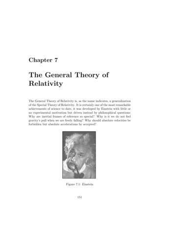
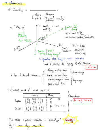
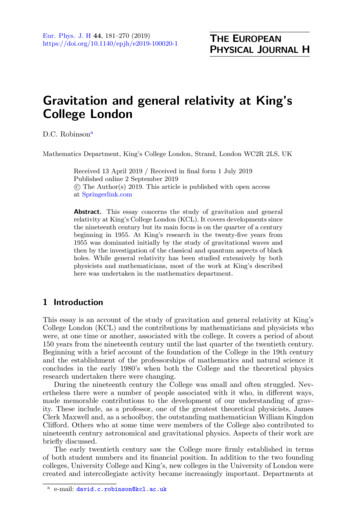
8CHAPTER 1. SPECIAL RELATIVITY Past of p: Set of all events for which t tp .More generally, we can define the future (past) of a set S to be the union of the futures(pasts) of all points of S.FUTUREPRESENTppPASTFigure 1.1: The Newtonian universe and its causal structureFrom now on we consider geometric units with respect to which the light travels atspeed c 1 relative to observers at rest. If an observer at p emits a light beam in alldirections of space, then the trajectory of this beam in spacetime will be a null cone withvertex at p. We can complete this cone by considering the trajectory of light beams thatarrive at the event p.FUTUREPRESENTpPASTFigure 1.2: The Newtonian universe and light trajectoriesIt is important to emphasize that in Newtonian theory, in view of the existence of theabsolute time t, one only works by projecting on the Euclidean space R3 and consideringall quantities as functions of (the space and) time t.Newton’s theory gives a very accurate theory for objects moving at slow speeds inabsence of strong gravitational fields. However, in several circumstances difficulties arise:1. A more philosophical issue is that in Newtonian theory an observer is either at restor in motion. But how could one determine if an observer O is (universally) at
1.2. THE BIRTH OF SPECIAL RELATIVITY9rest? Why can’t a uniformly moving (relative to O) observer P be considered atrest since P is also not affected by any external influence?2. For hundreds of years it has been known that in vacuum light propagates at a veryhigh but constant speed, and no material has been observed to travel faster. If anobserver P is moving at speed c/5 (relative to an observer O at rest) towards alight beam (which is moving at speed c relative to O), then the light would reachthe observer P at speed c c/5. However, astronomical observations of doublestars should reveal such fast and slow light, but in fact the speeds turn out to bethe same.3. Light is the propagation of an electromagnetic disturbance and electromagneticfields are governed by Maxwell’s equations. However, these equations are not wellbehaved in Newtonian theory; in particular, in this context, these laws are observerdependent and hence do not take the desired form of universal physical laws.One of Einstein’s contributions was his persistence that every physical law can beexpressed independently of the choice of coordinates (we will return to this point later).It was this persistence along with his belief that Maxwell’s equations are flawless thatled to what is now known as special relativity.1.2The Birth of Special RelativityIn 1905 Einstein published a paper titled “On the electrodynamics of moving bodies”,where he described algebraic relations governing the motion of uniform observers so thatMaxwell equations have the same form regardless of the observer’s frame. In order toachieve his goal, Einstein had to assume the following1. There is no absolute notion of time.2. No observer or particle can travel faster than the speed of light c. The constant cshould be considered as a physical law and hence does not depend on the observerwho measures it.The above immediately change the Newtonian perception for the spacetime, sinceunder Einstein’s assumptions the future (past) of an event p is confined to be the interiorof the future (past) light cone with vertex at p.
10CHAPTER 1. SPECIAL RELATIVITYIn 1908, Hermann Minkowski showed that Einstein’s algebraic laws (and, in particular, the above picture) can be interpreted in a purely geometric way, by introducing anew kind of metric on R4 , the so-called Minkowski metric.1.3The Minkowski Spacetime R3 1DefinitionA Minkowski metric g on the linear space R4 is a symmetric non-degenerate bilinearform with signature ( , , , ). In other words, there is a basis {e0 , e1 , e2 , e3 } such thatg(eα , eβ ) gαβ , α, β {0, 1, 2, 3} ,where the matrix gαβ is given by 1 0g 0001000010 00 .0 1Given such a frame (which for obvious reason will be called orthonormal), one can readilyconstruct a coordinate system (t, x1 , x2 , x3 ) of R4 such that at each point we havee0 t , ei xi , i 1, 2, 3.Note that from now on in order to emphasize the signature of the metric we will denotethe Minkowski spacetime by R3 1 . With respect to the above coordinate system, themetric g can be expressed as a (0,2) tensor as follows:g dt2 (dx1 )2 (dx2 )2 (dx3 )2 .(1.1)Note that (for an arbitrary pseudo-Riemannian metric) one can still introduce a Levi–Civita connection and therefore define the notion the associated Christoffel symbols andgeodesic curves and that of the Riemann, Ricci and scalar curvature. One can alsodefine the volume form such that if Xα , α 0, 1, 2, 3, is an orthonormal frame then (X0 , X1 , X2 , X3 ) 1. In the Minkowski case, the curvatures are all zero and thegeodesics are lines with respect to the coordinate system (t, x1 , x2 , x3 ).
1.3. THE MINKOWSKI SPACETIME R3 11.3.111Causality TheoryThe fundamental new aspect of this metric is that it is not positive-definite. A vectorX R3 1 is defined to be:1. spacelike, if g(X, X) 0,2. null, if g(X, X) 0,3. timelike, if g(X, X) 0.If X is either timelike or null, then it is called causal. If X (t, x1 , x2 , x3 ) is nullvector at p, thent2 (x1 )2 (x2 )2 (x3 )2and hence X lies on cone with vertex at p. In other words, all null vectors at p span adouble cone, known as the double null cone. We denote by Sp , Sp X Tp R3 1 : g(X, X) 0 ,the set of spacelike vectors at p, by Ip , Ip X Tp R3 1 : g(X, X) 0 ,the set of timelike vectors at p, and by Np , Np X Tp R3 1 : g(X, X) 0 ,the set of null vectors at p. The set Sp is open (and connected if n 1). Note that theset Ip is the interior of the solid double cone enclosed by Np . Hence, Ip is an open setconsisting of two components which we may denote by Ip and Ip . Then we can alsodecompose Np Np Np , whereNp Ip ,Np Ip .The following questions arise: How is Np (or Ip ) related to the future and past ofp? How can one even discriminate between the future and past? To answer this weneed to introduce the notion of time-orientability. A time-orientation of (R3 1 , g) is acontinuous choice of a positive component Ip at each p R3 1 . Then, we call Ip (resp.Np ) the set of future-directed timelike (resp. null) vectors at p. Similarly we define thepast-directed causal vectors. We also define: The causal future J (p) of p by J (p) Ip Np . The chronological future of p to simply be Ip .We also define the causal future J (S) of a set S by[J (S) Jp .p SCausality, observers and particles, proper time
12CHAPTER 1. SPECIAL RELATIVITYWe can readily extend the previous causal characterizations for curves. In particular,.a curve α : I R3 1 is called future-directed timelike if α(t) is a future-directed timelikevector at α(t) for all t I. Note that the worldline of an observer is represented by atimelike curve. If the observer is inertial, then he/she moves on a timelike geodesic. Onthe other hand, photons move on null geodesics (and hence information propagates alongnull geodesics).We, therefore, see that the Minkowski metric provides a very elegant way to put theassumptions of Section 1.2 in a geometric context.The proper time τ of an observer O is defined to be the parametrization of its worldline.α such that g(α(τ ), α(τ )) 1. Note that no proper time can be defined for photons.since for all parametrizations we have g(α(τ ), α(τ )) 0. However, in this case, it is.usually helpful to consider affine parametrizations τ with respect to which α. α 0.HypersurfacesFinally, we have the following categories for hypersurfaces:1. A hypesurface H is called spacelike, if the normal Nx at each point x H istimelike. In this case, gis positive-definite (i.e. H is a Riemannian manifold).Tx H2. A hypesurface H is called null, if the normal Nx at each point x H is null. Inthis case, gis degenerate.Tx H3. A hypesurface H is called timelike, if the normal Nx at each point x H is spacelike.In this case, ghas signature ( , , ).Tx HExamples of spacelike hypersurfaces1. The hypersurfacesHτ {t τ }
1.3. THE MINKOWSKI SPACETIME R3 113 are spacelike, since their unit normal is the timelike vector field 0 . Then, Hτ , g Tx Hτis isometric to the 3-dimensional Euclidean space E3 .2. The hypersurfaceH 3 {X : g(X, X) 1 and X future-directed }is a spacelike hypersurface. Indeed, one can easily verify that X is the normal toH 3 at the endpoint of X. Then, H 3 , gis isometric to the 3-dimensional3Tx Hhyperbolic space. The following figure depicts the radial projection which is anisometry from H 3 to the disk model.Note that the hyperboloid consists of all points in spacetime where an observerlocated at (0, 0, 0, 0) can be after proper time 1.We remark that the Cauchy–Schwarz inequality is reversed for timelike vectors. IfX, Y are two future-directed timelike vector fields then g(X, Y ) 0 and g(X, Y ) pg(X, X) · g(Y, Y ).Hence, there exists a real number φ such that g(X, Y )cosh(φ) p.g(X, X) · g(Y, Y )Then φ is called the hyperbolic angle of X and Y .Examples of timelike hypersurfaces1. The hypersurfacesTτ {x1 τ } are timelike, since their normal is the spacelike vector field x1 . Then, Tτ , gis isometric to the 3-dimensional Minkowski space R2 1 . Tx Tτ
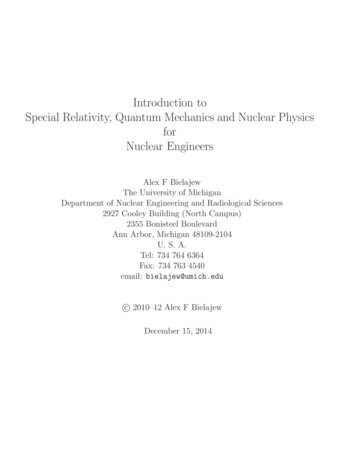
14CHAPTER 1. SPECIAL RELATIVITY2. The hypersurface3H {X : g(X, X) 1 and X future-directed }is a timelike hypersurface. Indeed, one can easily verify that X is the normal to3 at the endpoint of X.H Examples of null hypersurfaces1. Let n (n0 , n1 , n2 , n3 ) be a null vector. The planes given by the equation Pn (t, x1 , x2 , x3 ) : n0 t n1 x1 n2 x2 n3 x3are null hypersurfaces, since their normal is the null vector n.2. The (null) conenopC (t, x1 , x2 , x3 ) : t (x1 )2 (x2 )2 (x3 )2is also a null hypersurface. Its tangent plane at the endpoint of n is the plane Pnand hence its normal is the null vector n. Note that C N (O), where O is theorigin. Note also that N (O) is given byonpC (t, x1 , x2 , x3 ) : t (x1 )2 (x2 )2 (x3 )2 .The above can be summarized in the following figure:nullhypersurfacesictimelikehypersurfacenull geodetimelike geodesic inertial obesrverspacelikehypersurfacetimelike curve accelerating observer
1.3. THE MINKOWSKI SPACETIME R3 11.3.215Inertial Observers, Frames of Reference and IsometiesInertial FramesLet O be an inertial observer moving on a timelike geodesic α. Let t be the propertime of O and (x1 , x2 , x3 ) be a Euclidean coordinate system of the (spacelike) planeorthogonal to α at α(0). We will refer to the frame (t, x1 , x2 , x3 ) as the frame associatedto the inertial observer O.Relativity of TimeLet O0 be another (inertial or not) observer moving on the timelike curve α0 whichcan be expressed as α0 (τ ) (t(τ ), x1 (τ ), x2 (τ ), x3 (τ )) with respect to the frame associated to O. Note that since α0 is future-directed curve, the function t 7 t(τ ) isinvertible and hence we can write τ τ (t) giving us the following parametrizationα0 (t) (t, x1 (τ (t)), x2 (τ (t)), x3 (τ (t))). Note that the observer O at its proper time t sees0 (t) (x1 (τ (t)), x2 (τ (t)), x3 (τ (t))). Hence, the speed ofthat O0 is located at the point αOd 00O relative to O is dt αO (t) . As we shall see, we do not always have that t τ , in otherwords the time is relative to each observer. Let O0 be an inertial observer passing through the origin (0, 0, 0, 0) with respect tothe frame of O and also moving in the x1 -direction at speed v with respect to O. Then,O0 moves on the curve α0 (t) (t, vt, 0, 0); however, t is not the proper time of O0.since g(α(t), α(t)) 1 v 2 . However, if we consider the following parametrizationα0 (τ ) (γτ, γτ v, 0, 0), where1γ ,1 v2.0.0then τ is the proper time for O0 since g(α (τ ), α (τ )) 1. Note that γ cosh(φ),where φ is the hyperbolic angle of α(t 1) (1, 0, 0, 0) and α0 (τ 1).Time dilation: If τ is the proper time of O0 , then from the above representation weobtain that t γτ along α0 . Note that γ 1 and so t τ , which implies that the proper
16CHAPTER 1. SPECIAL RELATIVITYtime for the moving (with respect to O) observer O0 runs slower compared to the time tthat O measures for O0 .Isometries: Lorentz transformationsOne of the most striking properties of Minkowski spacetime is that there exists anisometry F which maps O to O0 . Relative to the frame associated to O this map takesthe form:F (t, x1 , x2 , x3 ) (γ · (t vx1 ), γ · (x1 vt), x2 , x3 ).ThenF [O(λ)] F (λ, 0, 0, 0) (γλ, γλv, 0, 0) α0 (λ) O0 (λ),where O(λ), O0 (λ) denotes the position of the observers O, O0 , respectively, at propertime λ. Clearly, the map F , being an isometry, leaves the proper time of observersinvariant.Note that although there is no absolute notion of time (and space consisting of simultaneous events), null cones are absolute geometric constructions that do not dependon observers (in particular, the isometry F leaves the null cones invariant).The isometry F is known as Lorentz transformation, or Lorentz boost in the x1 directionor hyperbolic rotation. The latter name arises from the fact that such an isometry can berepresented by a matrix whose form is similar to a Euclidean rotation but with trigonometric functions and angles replaced by hyperbolic trigonometric functions and angles.Note that the isometries F Fv (with v 2 1) correspond to the flow of the Killing fieldHx1 t x1 x1 t .Clearly, one can define boosts in any direction.Relativity of simultaneityHaving understood the relativity of time, we next proceed by investigating the relativity of space. The points simultaneous with observer O at the origin are all pointssuch that t 0. Then,F [{t 0}] F (0, x1 , x2 , x3 ) (γx1 v, γx1 , x2 , x3 ). We extend t0 such that {t0 0} F [{t 0}] and define the coordinates (x1 )0 , (x2 )0 , (x3 )0 on the hypersurface t0 0 such that if p {t0 0}, then p (x1 )0 , (x2 )0 , (x3 )0if F 1 (p) (0, x1 , x2 , x3 ). Note that the plane t0 0 consists of all points simultaneous with O0 at the origin and that one can define a global coordinate systemt0 , (x1 )0 , (x2 )0 , (x3 )0 . This is the reference frame associated to O0 . In view of thefact that F is an isometry,the metric takes the form (1.1) with respect to the system t0 , (x1 )0 , (x2 )0 , (x3 )0 .
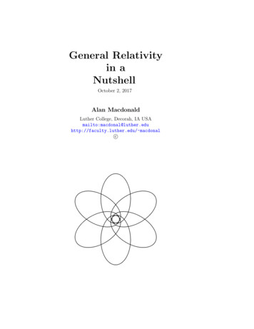
1.3. THE MINKOWSKI SPACETIME R3 117 Length Contraction: First note that distance between events is meaningful only forobservers who consider the events to be simultaneous. At proper time τ 1 of O0 ,observer O0 measures that his distance from observer O is v. However, when τ 1, themeasurements of O are such that O0 is located at the point (γ, γv, 0, 0) with respect tothe frame of O. Hence, the distance (after τ 1) that O measures between O and O0 isγv v. In other words, O0 measures shorter distances than O does. This phenomenonis called length contraction and is intimately connected to time dilation. OO Figure 1.3: The difference of the hyperbolic lengths of the blue (resp. red) segmentsrepresents length contraction (resp. time dilation).See also https://www.youtube.com/watch?v lVuF5zrwMLY.
18CHAPTER 1. SPECIAL RELATIVITY1.3.3General and Special CovarianceThe general covariance principle allows us to put physics in a geometric framework: General covariance principle: All physical laws are independent of the choiceof a particular coordinate system. In other words, the equations expressing physicallaws must be written in terms of tensors.Since the only tensor that we have in special relativity is the metric g, then we canin fact assume the following: Strong general covariance principle: All physical laws can be expressed interms of the metric g and its tensorial expressions.Hence, physical laws change covariantly (i.e. tensorially) under change of coordinates(i.e. under diffeomorphisms). If we apply this principle for Minkowski spacetime and alsorestrict to its isometries, then we obtain the following: Special covariance: The physical laws take exactly the same form when expressedin terms of the reference frames associated to inertial observers.1.3.4Relativistic Mechanics1. Time dilationWe will here generalize the result of the previous section on time dilation. Let Obe an inertial observer and O0 another (inertial or accelerating) observer. Let τ be theproper time of O0 such that his/her trajectory is α0 (τ ) (t(τ )), x1 (τ ), x2 , (τ ), x3 (τ )). Asbefore, we can write τ τ (t) and hence α0 (τ (t)) (t, x1 (τ (t), x2 (τ (t), x3 (τ (t)). If v is.0.0the speed of O0 relative to O, the fact that g(α (τ ), α (τ )) 1 implies thatdt1 1 t(τ ) τ.dτ1 v22. Absoluteness of speed of lightIf a particle moves of a null curve α0 (τ ) (t(τ )), x1 (τ ), x2 , (τ ), x3 (τ )) then the speedof the particle with respect to an inertial observer O isv 0dαOdτ 1,dτ dt.0.0where the last equation follows from g(α (τ ), α (τ )) 0.3. Energy-momentumLet α(τ ) represent the trajectory of a particle p with mass m. Then we have thefollowing definitions:
1.4. CONFORMAL STRUCTURE19. The 4-velocity of p is the vector U α(τ ) dαdτ . The energy-momentum of p is the vector P mU .Let’s now see how an inertial observer O measures the above quantities. If the particle pmoves at speed v relative to O, then by considering the frame associated to O, we obtain:P mdα dtmdα .2dt dτ1 v dt1. The spatial component of the energy-momentum vector P isPO mdαO,1 v 2 dtwhich is called the momentum of p as measured by O. (Compare this definitionwith the Newtonian definition in case v 0.)2. The temporal component of the energy-momentum vector P isEO 1m m mv 2 O(v 4 ),221 vwhich is called the total energy of p as measured by O. (Note, in particular, thatEO contains the kinetic energy 12 mv 2 ). Hence, the mass m is seen to be energy. Ifv 0, then energy of p as measured by a co-observer is E m, and by convertingin conditional units, we obtain Einstein’s famous equationE mc2 .1.4Conformal StructureOne is often interested in investigating the properties of isolated systems. In such situation one should only consider the local system and hence ignore the influence of matterat far distances. In other words, the asymptotic structure of the spacetime describingthe geometry of an isolated system should like the asymptotical structure of Minkowski(recall that Minkowski spacetime represents the geometry a vacuum static highly symmetric topologically trivial universe). The goal of this section is to describe the globaland asymptotic causal structure of Minkowski spacetimeOne could start by considering the following foliation of Minkowski:[R3 1 Hτ ,τ Rwhere the spacelike hypersurfaces Hτ {t τ } are as defined in Section 1.3. Note, however, this foliation does not capture the properties of null geodesics whose importanceis manifest from the fact that signals travel along such curves. Indeed, an observer (likeourselves on earth) located far away from an isolated system under investigation mustunderstand the asymptotic behavior of null geodesics in order to be able to measure
20CHAPTER 1. SPECIAL RELATIVITYradiation and other information sent from this system. For these reason, we will consider a foliation of Minkowski spacetime which captures the geometry of null geodesicsemanating from points of a timelike geodesic. This is the so-called double null foliation.As a final remark, note that since we want to understand the asymptotic structure, itwill be convenient to apply conformal transformations on Minkowski spacetime in orderto bring points at ‘infinity’ to finite distance. This procedure will allows us to reveal thestructure of infinity. Note that conformal transformations preserve the causal structure,since they send timelike curves to timelike curves, spacelike curves to spacelike curvesand null curves to null curves. In fact, conformal transformations send null geodesics tonull geodesics (see Section 2.2).1.4.1The Double Null FoliationLet us consider the timelike geodesic α(t) (t, 0, 0, 0) where the coordinates are takenwith respect to an inertial coordinate system (t, x1 , x2 , x3 ). Recall that the futuredirected null cone CO with vertex at O α(0) is given bynop1 2 3122232C0 (t, x , x , x ) : t (x ) (x ) (x ) 0 ,whereas the past-directed null cone C O with vertex at O α(0) is given bynopC 0 (t, x1 , x2 , x3 ) : t (x1 )2 (x2 )2 (x3 )2 0 .In order to simplify the above expressions and capture the spherical symmetry of thenull cones, it is convenient to introduce spherical coordinates (r, θ, φ) for the Euclideanhypersurfaces Hτ such that r 0 corresponds to the curve α. Then, in (t, r, θ, φ)coordinates, the Minkowski metric takes the formg dt2 dr2 r2 · gS2 (θ,φ) ,where gS2 (θ, φ) dθ2 (sin θ)2 dφ2 is the standard metric on the unit sphere. Then thefuture-directed null cone Cτ with vertex at α(τ ) is given byCτ {(t, r, θ, φ) : t r τ, τ R} ,whereas the past-directed null cone C τ with vertex at α(τ ) is given byC τ {(t, r, θ, φ) : t r τ, τ R} .The above suggest that it is very convenient to convert to null coordinates (u, v, θ, φ)defined such thatu t r,v t r.Note also thatv u(1.2)
1.4. CONFORMAL STRUCTURE21and v u if and only if r 0. The metric with respect to null coordinates (u, v, θ, φ)takes the form1g dudv (u v)2 · gS2 (θ,φ)4and the double null folation is given by the equationsCτ {(u, v, θ, φ) : u τ, τ R} ,C τ {(u, v, θ, φ) : v τ, τ R} .Note that v (resp. u ) is tangential to the null geodesics of the null cones Cτ (resp.C τ ). For a generalization of the double null foliation see Section 4.1.1.4.2The Penrose DiagramThe aim of the section is to describe the asymptotic structure of Minkowski space. Inparticular, we want to draw a “bounded” diagram whose boundary represents infinityand somehow respects the causal structure of Minkowski.Clearly, v along the null cones Cτ and similarly u along the null conesC τ . In order to bring the endpoint of null geodesics in finite distance, we consider thefollowing change of coordinates:tan p v,tan q u,with p, q π π2, 2 (1.3)and p q. Then in (p, q, θ, φ) coordinates the metric takes the form 112g dp dq sin (p q) · gS2 (θ,φ) .(cos p)2 · (cos q)24
22CHAPTER 1. SPECIAL RELATIVITYAs expected, a consequence of the boundedness of the range of p, q is that the factor1blows up as p π2 or q π2 . In order to overcome this degeneracy, we(cos p)2 ·(cos q)2consider the metric g̃ which in (p, q, θ, φ) takes the formg̃ dp dq 1sin2 (p q) · gS2 (θ,φ) .4(1.4)Clearly the metric g̃ is conformal to g. Note that p q , q p , where the isconsidered with respect to g̃, and therefore, the hypersurfaceseτ {(p, q, θ, φ) : q τ, τ R} ,Ce τ {(p, q, θ, φ) : p τ, τ R} .Care null (with respect to g̃). Hence, if we suppress one angular direction, we can globallyf g̃) covered by
Chapter 1 Special Relativity In both past and modern viewpoints, the universe is considered to be a continuum composed of events, where each event can be thought of as a point in space at an instant