Transcription
EPA 600/R-?/?December 2008www.epa.govWASP8 TemperatureModel Theory and User’s GuideSupplement to Water Quality AnalysisSimulation Program (WASP) UserDocumentationTim A. WoolU.S. EPA, Region 4Water Management DivisionAtlanta, GeorgiaRobert B. Ambrose, Jr., P.E.U.S. EPA, Office of Research and DevelopmentNational Exposure Research LaboratoryEcosystems Research DivisionAthens, GeorgiaJames L. Martin, Ph.D., P.E.Mississippi State UniversityStarkville, MississippiU.S. Environmental Protection AgencyOffice of Research and DevelopmentWashington, DC 20460
User’s GuideWASP Temperature ModuleNOTICEThe U.S. Environmental Protection Agency (EPA) through its Office of Research and Development(ORD) funded and managed the research described herein. It has been subjected to the Agency’speer and administrative review and has been approved for publication as an EPA document. Mentionof trade names or commercial products does not constitute endorsement or recommendation for use.i
User’s GuideWASP Temperature ModuleABSTRACTThe standard WASP eutrophication and toxicant modules use water temperature to determine ratesof reactions that are influenced by temperature. In many cases there is not enough spatial andtemporal water temperature data to adequately parameterize a water quality model. The WASPTemperature Module can be used to predict water column temperature based upon atmosphericconditions and heat exchange between the surface, subsurface and benthic layers of the water body.Furthermore, WASP has methods for transferring the predicted water temperatures to other WASPsub models via a transfer interface file.This supplemental user manual documents the temperature algorithms, including the kineticequations, the additional model input and output, and a series of model verification tests.ii
User’s GuideWASP Temperature ModuleTable of Contents1Introduction . 12Model Theory. 22.1General Mass Balance Equation . 22.2Water Quality Kinetics . 32.2.134Temperature . 3Model Input. 133.1Model Parameters . 133.2Model Constants . 153.3Kinetic Time Functions . 17References. 21List of FiguresFigure 1 Segment Parameters for Temperature Module . 13Figure 3 Global Constants for the Temperature Module . 15Figure 4 Constants for Temperature Calculation. 16Figure 5 Constants for Fecal Coliform Calculation . 17Figure 6 Kinetic Time Functions for Temperature Module . 18List of Tablesiii
User’s GuideWASP Temperature ModuleTable 1 Description of Segment Parameters for Temperature Module . 14Table 2 Global Constants for Heat Module of WASP . 15Table 3 Temperature Kinetic Constants for Heat Module of WASP . 17Table 4 Fecal Coliform Kinetic Constants . 17Table 5 Environmental Time Functions for the Temperature Module . 19iv
User’s GuideWASP Temperature Module1IntroductionThe Water Analysis Simulation Program (WASP, Ambrose et al 1993) is a dynamic compartmentmodeling system that can be applied to a variety of water bodies. The flexibility afforded by WASPis unique. WASP permits the modeler to structure one, two, and three dimensional models; allowsthe specification of time-variable exchange coefficients, advective flows, waste loads and waterquality boundary conditions.One of the other unique advantages to WASP is its modular structure which permits tailingstructuring of the kinetic processes, all within the larger modeling framework without having towrite or rewrite large sections of computer code. The two primary operational WASP models,toxicants and eutrophication, are reasonably general and are intended to simulate two of the majorclasses of water quality problems: conventional pollution (involving dissolved oxygen, biochemicaloxygen demand, nutrients and eutrophication) and toxic pollution (involving organic chemicals andsediment). In addition, kinetic models have been developed for mercury (MERC4, Martin 1992) andfor simulation of metals in general (META4, Martin and Medine 1996).With the release of WASP8 the capability of simulating water temperatures has been added to boththe toxicant and eutrophication module. Temperatures affect many of the kinetic rates in all versionsof WASP and are often important in their own right. WASP8 has been developed to allow thedynamic simulation of processes affecting water temperatures, including surface heat exchange, iceformation and breakup. The temperature routines are based upon those in the U.S. Army Corps ofEngineers CE-QUAL-W2 model (Hydraulics and Environmental Laboratories 1984, Cole andBuchak 1994).This manual is intended to describe the basic relationships used to predict variations in each of thefive state variables simulated by Heat Module as well as describe the model input requirements.This manual is intended as supplement to the WASP manual (Ambrose et al 1993), and the reader isreferred to that manual for a more complete description of WASP model theory and inputrequirements. In addition, the basic relationships used to predict temperature variations, asdescribed in the following section, were taken from Cole and Buchak (1995).1
User’s GuideWASP Temperature Module22.1Model TheoryGeneral Mass Balance EquationThe basic equations solved by all versions of WASP are those based upon laws of conservation.The primary laws of conservation used in the development of water quality models include those forenergy, mass and momentum. For example, the hydrodynamic models DYNHYD and RIVMOD arebased upon conservation of momentum and water mass. Previous versions of WASP were basedupon the conservation of water and constituent mass. The Heat Module model is also based uponconservation of water and constituent mass (for salinity, coliform bacteria, and the arbitraryconstituents), as well as the law of conservation of energy, for heat transfer. These laws form theunderlying principals of much of modern science and engineering as well as water quality modeling.For all materials that act according to the laws of conservation, if some transformation or changeoccurs, the total amount of the material present after the change or transformation must be identicalto that present before. For mass, in order to account for processes affecting the transformation thebalance equation must account for material entering and leaving through direct and diffuse loading;advective and dispersive transport; and physical, chemical, and biological transformations. For acoordinate system where the x- and y-coordinates are in the horizontal plane and the z-coordinate isin the vertical plane, the mass balance equation around an infinitesimally small fluid volume is: C ( U x C) ( U y C) ( U z C) t x y z C C C(Ex) (E y) (Ez) x x y y z z S L S B S Kwhere:C concentration of the water quality constituent, mg/L or g/m3t time, daysUx,Uy,Uz longitudinal, lateral, and vertical advective velocities, m/dayEx,Ey,Ez longitudinal, lateral, and vertical diffusion coefficients, m2/daySL direct and diffuse loading rate, g/m3-daySB boundary loading rate (including upstream, downstream, benthic, andatmospheric), g/m3-day2
User’s GuideWASP Temperature ModuleSKg/m3-day total kinetic transformation rate; positive is source, negative is sink,The mass balance equation as written above is based upon constituent concentrations, which refersto the mass of that dissolved or suspended in a given volume of water. Similarly, temperature maybe considered a measure of the amount of heat energy contained in a volume of water, and therelationship between heat energy and temperature is given by:H V w C P T V C hwhere H is the heat content, Cp the specific heat of water (at a given pressure) and T thetemperature, where the quantity in parenthesis may be considered the "concentration" of heat (C h).Replacing the constituent concentration with the heat concentration in the above equation results inthe heat balance equation, which is solved by Heat Module for water temperatures.By expanding the infinitesimally small control volumes into larger adjoining "segments," and byspecifying proper transport, loading, and transformation parameters, WASP implements afinite-difference form of equation (. The basic equation is applied to a set of expanded controlvolumes, or "segments," that together represent the physical configuration of the water body. Thenetwork may subdivide the water body laterally and vertically as well as longitudinally. Benthicsegments can be included along with water column segments. If the water quality model is beinglinked to the hydrodynamic model, then water column segments must correspond to thehydrodynamic junctions. Concentrations of water quality constituents and temperatures arecalculated within each segment. Transport rates of water quality constituents are calculated acrossthe interface of adjoining segments.2.2Water Quality KineticsThe balance relationship described in the previous section is solved by WASP for all state variables.The basic relationship is the same regardless of the state variable. Differences occur betweenWASP submodels in the number of state variables and the in the processes which are included in thetotal kinetic transformation rate (SK) for each state variable. All versions of WASP share the samemain program, which computes all terms except for SK. That term is computed in a separate module(WASPB) which is specific to the submodel (EUTRO, TOXI).2.2.1TemperatureThe processes included in the total transformation rates for temperature include surface and bottomheat exchange. Surface heat exchange is calculated by either a full heat balance or of through use of3
User’s GuideWASP Temperature Moduleequilibrium temperatures and coefficients of surface heat exchange (Brady and Edinger, 1975). Thesurface heat budget is described below and is taken from Cole and Buchak (1994).2.2.1.1Surface Heat ExchangeThe source and sink term for heat includes loadings from external sources, such as thermaldischarges, as well as heat exchange across the air-water interface. The sources and sinks term forwater temperature due to surface heat exchange may be written as V TH A exchange n s t Cpwhere V is volume (m3), As is surface area (m2), T is temperature (oC), t is time, ρ the density ofwater (997 Kg m-3 at 25 oC), Cp is its specific heat (4179 J Kg-1 oC-1 at 25oC), and Hn (Watts m-2) isthe net thermal energy flux. The net thermal energy flux includes the effects of a number ofprocesses. The net thermal energy flux (Hn, Watts m-2), may be expressed asTerm-by-term surface heat exchange is computed as:Hn Hs Ha He Hc - ( Hsr Har Hbr )whereHnHsHaHsrHarHbrHeHc the net rate of heat exchange across the water surface, W m-2incident short wave solar radiation, W m-2incident long wave radiation, W m-2reflected short wave solar radiation, W m-2reflected long wave radiation, W m-2back radiation from the water surface, W m-2evaporative heat loss, W m-2heat conduction, W m-2In Heat Module, the surface heat exchange processes depending on water surface temperatures arecomputed using previous time step data and are therefore lagged from transport processes by themodel time step. The short wave solar radiation (Hs) is either measured directly or computed fromsun angle relationships and cloud cover. The long wave atmospheric radiation is computed from airtemperature and cloud cover or air vapor pressure using Brunts formula.4
User’s GuideWASP Temperature ModuleWater surface back radiation is computed from:4*H br (Ts 273.15)Whereεσ*Ts emissivity of water, 0.97Stephan-Boltzman constant, 5.67 x 10⁻⁸ W m-2 K-4water surface temperature, CEvaporative heat loss is computed as:He f(W) (es - ea )wheref(W)esea evaporative wind speed function, W m-2 mm Hg-1saturation vapor pressure at the water surface, mm Hgatmospheric vapor pressure, mm HgEvaporative heat loss depends on air temperature and dew point temperature or relative humidity.Surface vapor pressure is computed from the surface temperature for each surface segment.Surface heat conduction is computed as:Hc Cc f(W) (Ts - Ta )whereCcTa Bowen's coefficient, 0.47 mm Hg C-1air temperature, CShort wave solar radiation penetrates the surface and decays exponentially with depth according toBears Law:- zHs (z) (1 - ) Hs eWhereHs(z) short wave radiation at depth z, W m-25
User’s GuideWASP Temperature ModuleβηHs fraction absorbed at the water surfaceextinction coefficient, m-1short wave radiation reaching the surface, W m-2In the equilibrium temperature approach, a temperature is computed at which the net surfaceexchange is equal to zero. The linearization of the net heat balance and this definition of theequilibrium temperature allows the net rate of surface heat exchange, Hn, to be expressed as:Hn - K aw (T w - Te )whereHnKawTwTe rate of surface heat exchange, W m-2coefficient of surface heat exchange, W m-2 C-1water surface temperature, Cequilibrium temperature, CSeven separate heat exchange processes are summarized in the coefficient of surface heat exchangeand equilibrium temperature. The linearization used in obtaining equation ( has been examined indetail by Brady, et al. (1968), and Edinger et al. (1974).2.2.1.2Sediment Heat ExchangeSediment heat exchange with water is generally small compared to surface heat exchange and hasoften been neglected. However, investigations on several reservoirs have shown the process must beincluded to accurately reproduce hypolimnetic temperatures primarily because of the reduction innumerical diffusion (Cole and Buchak 1994). The formulation used to compute bottom heat transferis similar to that used in the equilibrium temperature approach for surface exchange:Hsw - Ksw (T w - Ts )Where:HswKswTwTs rate of sediment/water heat exchange, W m-2coefficient of sediment/water heat exchange, W m-2 C-1water temperature, Csediment temperature, CCole and Buchak (1994) indicated that values of 7 x 10⁻⁸ W m-2 C-1 for Ksw have been used inprevious applications and that average yearly air temperature is a good estimate of T s.6
User’s GuideWASP Temperature Module2.2.1.3Ice CoverIce formation can affect the heat balance, mixing characteristics, and water quality in lakes andreservoirs. For example, once a lake freezes over, sensible heat losses and evaporation nearly ceaseand net radiation is strongly outward, resulting in more or less steady ice growth during early wintermonths (Lerman 1978). In addition, other processes which are often negligible during ice-freeperiods, such as heat flux from the bottom, become important in the heat cycle. Ice essentiallyshields the lake against wind mixing and retards light penetration, depending upon the thickness ofthe ice and snow cover. Surface reaeration is also retarded during periods of ice cover and in manyshallow eutrophic lakes anoxic conditions often occur following long periods of ice and snow coverand may result in winter fish kills.Ice cover is described to the eutrophication submodel of WASP. Heat Module computes ice cover,based on relationships included in the CE-QUAL-W2 model (Cole and Buchak 1994). The icemodel is based on an ice cover with ice-to-air heat exchange, conduction through the ice, conductionbetween underlying water, and a "melt temperature" layer on the ice bottom (Cole and Buchak 1994,Ashton, 1979). The overall heat balance for the water-to-ice-to-air system is: i Lf h h ai (T i - T e ) - h wi (T w - T m ) twhereρiLfΔh/ΔthaihwiTiTeiTwTm density of ice, kg m-3latent heat of fusion of ice, J kg-1change in ice thickness (h) with time (t), m sec-1coefficient of ice-to-air heat exchange, W m-2 C-1coefficient of water-to-ice heat exchange through the melt layer, W m-2 C-1ice temperature, Cequilibrium temperature of ice-to-air heat exchange, Cwater temperature below ice, Cmelt temperature, 0 CThe ice-to-air coefficient of surface heat exchange, hai, and its equilibrium temperature, Tei, arecomputed the same as for surface heat exchange in Edinger, et al. (1974) because heat balance of thethin, ice surface water layer is the same as the net rate of surface heat exchange presented previously. The coefficient of water-to-ice exchange, hwi, depends on turbulence and water movementunder ice and their effect on melt layer thickness. It is a function of water velocity for rivers butmust be empirically adjusted for reservoirs.Ice temperature in the ice-heat balance is computed by equating the rate of surface heat transferbetween ice and air to the rate of heat conduction through ice:7
User’s GuideWASP Temperature Module-k i (T i - T m )h ai (T i - T ei ) hwhereki molecular heat conductivity of ice, W m-1 C-1When solved for ice temperature, Ti, and inserted in the overall ice-heat balance, the ice thicknessrelationship becomes: i Lf h t() T M T ei - h wi (T w - T m )h1 kih iafrom which ice thickness can be computed for each longitudinal segment. Heat from water to icetransferred by the last term is removed in the water temperature transport computations.Variations in the onset of ice cover and seasonal growth and melt over the waterbody depend onlocations and temperatures of inflows and outflows, evaporative wind variations over the ice surface,nd effects of water movement on the ice-to-water exchange coefficient. Ice will often form inreservoir branches before forming in the main pool and remain longer due to these effects.A second, more detailed algorithm for computing ice growth and decay has been developed for CEQUAL-W2 (Cole and Buchak 1994) and is include in Heat Module. The algorithm consists of aseries of one-dimensional, quasi steady-state, thermodynamic calculations for each time step. It issimilar to those of Maykut and Untersteiner (1971), Wake (1977) and Patterson and Hamblin (1988).The detailed algorithm provides a more accurate representation of the upper part of the icetemperature profile resulting in a more accurate calculation of ice surface temperature and rate of icefreezing and melting.The ice surface temperature, Ts, is iteratively computed at each time step using the upper boundarycondition as follows. Assuming linear thermal gradients and using finite difference approximations,heat fluxes through the ice, qi, and at the ice-water interface, qiw, are computed. Ice thickness attime t, θ(t), is determined by ice melt at the air-ice interface, Δθai, and ice growth and melt at theice-water interface, Δθiw. The computational sequence of ice cover is presented below.Initial ice formation. Formation of ice requires lowering the surface water temperature to thefreezing point by normal surface heat exchange processes. With further heat removal, ice begins toform on the water surface. This is indicated by a negative water surface temperature. The negativewater surface temperature is then converted to equivalent ice thickness and equivalent heat is addedto the heat source and sink term for water. The computation is done once for each segment8
User’s GuideWASP Temperature Modulebeginning with the ice-free period: 0 -T w n w C P w h i Lfwhereθ0Twn thickness of initial ice formation during a time step, mlocal temporary negative water temperature, ChρwCpwρiLf layer thickness, mdensity of water, kg m-3specific heat of water, J kg-1 C-1density of ice, kg m-3latent heat of fusion, J kg-1Upper air-ice interface flux boundary condition and ice surface temperature approximation: The icesurface temperature, Ts, must be known to calculate the heat components, Hbr, He, Hc, and the thermal gradient in the ice since the components and gradient all are either explicitly or implicitly afunction of Ts. Except during the active thawing season when ice surface temperature is constant at0 C, Ts must be computed at each time step using the upper boundary condition. The approximatevalue for Ts is obtained by linearizing the ice thickness across the time step and solving for Ts.qi KiT f - T s(t) (t)Hsn H an - H br - H e - H c q i i LfnTs n-1Kid ai, for T s 0 o Cdtnn H an- H br T sn - H e T sn - H c T sn H snwhereKiTfn thermal conductivity of ice, W m-1 C -1freezing point temperature, Ctime level9
User’s GuideWASP Temperature ModuleAbsorbed solar radiation by the water under the ice. Although the amount of penetrated solarradiation is relatively small, it is an important component of the heat budget since it is the only heatsource to the water column when ice is present and may contribute significantly to ice melting at theice-water interface. The amount of solar radiation absorbed by water under the ice cover may beexpressed as:- (t)H ps Hs (1- ALBi) (1- i) e iwhereHpsHsALBiβiγi solar radiation absorbed by water under ice cover, W m-2incident solar radiation, W m-2ice albedofraction of the incoming solar radiation absorbed in the ice surfaceice extinction coefficient, m-1Ice melt at the air-ice interface. The solution for Ts holds as long as net surface heat exchange,Hn(Ts), remains negative corresponding to surface cooling, and surface melting cannot occur. IfHn(Ts) becomes positive corresponding to a net gain of heat at the surface, qi must become negativeand an equilibrium solution can only exist if Ts Tf. This situation is not possible as melting willoccur at the surface before equilibrium is reached (Patterson and Hamblin, 1988). As a result ofquasi-steady approximation, heat, which in reality is used to melt ice at the surface, is storedinternally producing an unrealistic temperature profile. Stored energy is used for melting at eachtime step and since total energy input is the same, net error is small. Stored energy used for meltingice is expressed as:(t) i Cp T s (t) i Lf aii2whereCpiθa1 specific heat of ice, J kg-1 C-1ice melt at the air-ice interface, m-1Formulation of lower ice-water interface flux boundary condition. Both ice growth and melt mayoccur at the ice-water interface. The interface temperature, Tf, is fixed by the water properties. Fluxof heat in the ice at the interface therefore depends on Tf and the surface temperature Ts through theheat flux qi. Independently, heat flux from the water to ice, qiw, depends only on conditions beneaththe ice. An imbalance between these fluxes provides a mechanism for freezing or melting. Thus,10
User’s GuideWASP Temperature Moduleq i - q iw i Lfd iwdtwhereθiw ice growth/melt at the ice-water interfaceThe coefficient of water-to-ice exchange, Kwi, depends on turbulence and water movement underthe ice and their effect on melt layer thickness. It is known to be a function of water velocity forrivers and streams but must be empirically adjusted for reservoirs. The heat flux at the ice-waterinterface is:q iw h wi T w(t) - Tf whereTw water temperature in the uppermost layer under the ice, CFinally, ice growth or melt at the ice-water interface is: 2.2.1.4niw n Tf - Ts nKih wi (T w - T f ) n-1 i Lf 1DensityWater densities are affected by variations in temperature and solids concentrations given by : T SwhereρρTΔρS density, kg m-3water density as a function of temperature, kg m-3density increment due to solids, kg m-3A variety of formulations have been proposed to describe water density variations due totemperatures. The following relationship is used in Heat Module (Cole and Buchak 1994,Gill,1982):11
User’s GuideWASP Temperature Module T 999.8452594 6.793952 x 10⁻² T ww- 9.095290 x 10⁻³ T 2w 1.001685 x 10⁻⁴ T 3w- 1.120083 x 10⁻⁶ T 4w 6.536332 x 10⁻⁹ x T 5wThe affect of dissolved solids, expressed as either salinity or total dissolved solids, on density isalso included. Density effects due to TDS is given by Ford and Johnson (1983): TDS (8.221x 10⁻⁴ - 3.87 x 10⁻⁶ T w 4.99 x 10⁻⁸ T 2w) TDSwhereΦTDS TDS concentration, g m-3and for salinity (Gill, 1982): sal (0.824493 - 4.0899 x 10⁻³ T w 7.6438 x 10⁻⁵ T 2w- 8.2467 x 10⁻⁷ T 3w 5.3875 x 10⁻⁹ T 4w ) sal (-5.72466 x 10⁻³ 1.0227 x 10⁻⁴ T w-42- 1.6546 x 10⁻⁶ T 2w ) 1.5sal 4.8314 x 10 salwhere3Φsal salinity, kg m-312
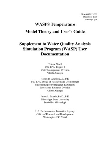
User’s GuideWASP Temperature Module3Model InputThe data required to support the application of a model of the thermal module include initialconditions (segment parameters, environmental time functions and kinetic constants. Eachof these is briefly described in the sections below.3.1Model ParametersParameters are spatially-variable characteristics of the water body. The definition of theparameters will vary, depending upon the structure and kinetics of the systems comprisingeach model. The input format, however, is constant. The number of parameters that isspecified must be input for each segment. Figure 1 and illustrate where the user woulddefine and enable segment specific parameters. If a segment parameter is not defined by theuser, it is considered to be inactive.Figure 1 Segment Parameters for Temperature ModuleNot only does the used have to define the segment specific parameters, the user must enablethe parameter and adjust the scale factor if need be.Table 1 provides a detailed description of the segment parameters that are available for theheat module.13
User’s GuideWASP Temperature ModuleTable 1 Description of Segment Parameters for Temperature ModuleDescriptionNamePointer to Cloud Cover TimeFunctionCloud Cover Multiplier (unitlessor fraction)Pointer to Wind Speed TimeFunctionWind Speed Multiplier (unitlessor m/sec)Pointer to Air Temperature TimeFunctionAir Temperature Multiplier(unitless or C)Pointer to Dew Point TimeFunctionDew Point TemperatureMultiplier (unitless or C)Flag designating the time-variable cloud cover function to be used forthe segment. The four cloud cover time functions are defined by the userin the Environmental Time Function Data Entry ScreenSegment clouds cover multiplier. Cloud Cover varies over space andcan be either actual cloud cover (as a percent of clear sky) or anormalized function, depending on the way the user defines the timefunction.Flag designating the time-variable wind speed function to be used for thesegment. The four wind speed functions are defined the EnvironmentalTime Function Data Entry Screen.Segment wind speed multiplier. Wind speed varies over space and can beeither wind speed (m/sec) or a normalized function, depending on theway the user defines the time function.Flag designating the time-variable air temperature function to be usedfor the segment. The air temperature functions are defined theEnvironmental Time Function Data Entry Screen.Segment air temperature multiplier. Air Temperature varies over spaceand can be either air temperature ( 0C) or a normalized function,depending on the way the user defines the time function.Flag designating the time-variable dew point temperature function to beused for the segment. The dew point temperature functions are definedthe Environmental Time Function Data Entry Screen.Segment dew point temperature multiplier. Segment Dew Point Multipliervaries over space and can be either the dew point temperature (0C) or anormalized function, depending on the way the user defines the timefunction.Wind Sheltering CoefficientMultiplier (unitless or fraction)Segment wind sheltering coefficient multiplier (a fraction, from 0 to 1).The wind sheltering coefficient varies over space and can be either anactual sheltering coefficient or a normalized function, depending on thedefinition.Pointer to Wind Sheltering TimeFunctionPointer designating the time variable wind sheltering coefficient to beused for segment. This coefficient is used to adjust the effects of thewind. Its physical basis is that surrounding terrain often shelters thewaterbody so that observed winds taken from meteorological stations arenot the effective winds reaching the waterbody. Since prevailing winddirection and vegetative cover vary with time, the user has the option tovary the wind sheltering coefficient with time as well as space. The foursheltering coefficients time functions available are defined in theEnvironmental Time Function Data Entry Screen.Light Extinction CoefficientMultiplier (unitless or 1/m)Segment extinction coefficient multiplier (m-1). Light Extinction variesover space and can be either an actual extinction coefficient or anormalized function, depending on the definition.14
User’s GuideWASP Temperature Module3.2Model ConstantsThe definition
total kinetic transformation rate; positive is source, negative is sink, g/m3-day The mass balance equation as written above is based upon constituent concentrations, which refers to the mass of that dissolved or suspend