Transcription
Printed Page 191SECTION 3.2 Exercises and Solutions35.What’s my line? You use the same bar of soap to shower each morning. Thebar weighs 80 grams when it is new. Its weight goes down by 6 grams per dayon the average. What is the equation of the regression line for predictingweight from days of use?Correct AnswerThe equation is ŷ 80 6x where ŷ the estimated weight of the soap and x thenumber of days since the bar was new.36.37.What’s my line? An eccentric professor believes that a child with IQ 100should have a reading test score of 50, and that reading score shouldincrease by 1 point for every additional point of IQ. What is the equation ofthe professor’s regression line for predicting reading score from IQ?Gas mileage We expect a car’s highway gas mileage to be related to its citygas mileage. Data for all 1198 vehicles in the government’s 2008 FuelEconomy Guide give the regression line predicted highway mpg 4.62 1.109 (city mpg). (a) What’s the slope of this line? Interpret this value in context. (b) What’s the intercept? Explain why the value of the intercept is notstatistically meaningful. (c) Find the predicted highway mileage for a car that gets 16 milesper gallon in the city. Do the same for a car with city mileage 28mpg.Correct Answer(a) The slope is 1.109. We predict highway mileage will increase by 1.109 mpg foreach 1 mpg increase in city mileage. (b) The intercept is 4.62 mpg. This is notstatistically meaningful, because this would represent the highway mileage for a carthat gets 0 mpg in the city. (c) With city mpg of 16, the predicted highway mpg is4.62 1.109(16) 22.36 mpg. With city mpg of 28, the predicted highway mpg is4.62 1.109(28) 35.67 mpg.38.IQ and reading scores Data on the IQ test scores and reading test scoresfor a group of fifth-grade children give the following regression line:predicted reading score 33.4 0.882(IQ score). (a) What’s the slope of this line? Interpret this value in context.
39.pg 166 (b) What’s the intercept? Explain why the value of the intercept is notstatistically meaningful. (c) Find the predicted reading scores for two children with IQ scoresof 90 and 130, respectively.Acid rain Researchers studying acid rain measured the acidity ofprecipitation in a Colorado wilderness area for 150 consecutive weeks.Acidity is measured by pH. Lower pH values show higher acidity. Theresearchers observed a linear pattern over time. They reported that theregression line(weeks) fit the data well.16 (a) Identify the slope of the line and explain what it means in thissetting. (b) Identify the y intercept of the line and explain what it means inthis setting. (c) According to the regression line, what was the pH at the end ofthis study?Correct Answer(a) The slope is 0.0053; the pH decreased by 0.0053 units per week on average.(b) The y intercept is 5.43, and it provides an estimate for the pH level at thebeginning of the study. (c) The pH is predicted to be 4.635 at the end of the study.40.How much gas? In Exercise 4 (page 158), we examined the relationshipbetween the average monthly temperature and the amount of natural gasconsumed in Joan’s midwestern home. The figure below shows the originalscatterplot with the least-squares line added. The equation of the leastsquares line is.
41. (a) Identify the slope of the line and explain what it means in thissetting. (b) Identify the y intercept of the line. Explain why it’s risky to usethis value as a prediction. (c) Use the regression line to predict the amount of natural gas Joanwill use in a month with an average temperature of 30 F.Acid rain Refer to Exercise 39. Would it be appropriate to use theregression line to predict pH after 1000 months? Justify your answer.Correct AnswerNo. The data was collected weekly for 150 weeks. 1000 months corresponds toroughly 4000 weeks, which is well outside the observed time period. This constitutesextrapolation.42.43.How much gas? Refer to Exercise 40. Would it be appropriate to use theregression line to predict Joan’s natural-gas consumption in a future monthwith an average temperature of 65 F? Justify your answer.Least-squares idea The table below gives a small set of data. Which of thefollowing two lines fits the data better:orMake a graph ofthe data and use it to help justify your answer. (Note: Neither of these twolines is the least-squares regression line for these data.)
Correct AnswerThe dotted line in the scatterplot is the line ŷ 1 x and the solid line is the line ŷ 3 2x. The dotted line comes closer to all the data points. Thus, the line ŷ 1 x fits the data better.44.45.pg 168Least-squares idea Trace the graph from Exercise 40 on your paper.Show why the line drawn on the plot is called the least-squares line.Acid rain In the acid rain study of Exercise 39, the actual pHmeasurement for Week 50 was 5.08. Find and interpret the residual for thisweek.Correct AnswerThe residual is 0.085. The line predicted a pH value for that week that was 0.085too large.46.47.pg 173How much gas? Refer to Exercise 40. During March, the averagetemperature was 46.4 F and Joan used 490 cubic feet of gas per day. Findand interpret the residual for this month.Husbands and wives The mean height of American women in their earlytwenties is 64.5 inches and the standard deviation is 2.5 inches. The meanheight of men the same age is 68.5 inches, with standard deviation 2.7inches. The correlation between the heights of husbands and wives is aboutr 0.5. (a) Find the equation of the least-squares regression line forpredicting husband’s height from wife’s height. Show your work. (b) Use your regression line to predict the height of the husband of awoman who is 67 inches tall. Explain why you could have given thisresult without doing the calculation.Correct Answer
(a) The equation for predicting y husband’s height from x wife’s height is ŷ 33.67 0.54x. (b) The predicted height is 69.85 inches. 67 inches is one standarddeviation above the mean for women. So the predicted value for husband’s heightwould be.48.49.The stock market Some people think that the behavior of the stock marketin January predicts its behavior for the rest of the year. Take theexplanatory variable x to be the percent change in a stock market index inJanuary and the response variable y to be the change in the index for theentire year. We expect a positive correlation between x and y because thechange during January contributes to the full year’s change. Calculationfrom data for an 18-year period gives (a) Find the equation of the least-squares line for predicting full-yearchange from January change. Show your work. (b) The mean change in January is. Use your regression lineto predict the change in the index in a year in which the index rises1.75% in January. Why could you have given this result (up toroundoff error) without doing the calculation?Husbands and wives Refer to Exercise 47. (a) Find r2 and interpret this value in context. (b) For these data, s 1.2. Explain what this value means.Correct Answer(a) r2 0.25. Thus, the straight-line relationship explains 25% of the variation inhusbands’ heights. (b) The average error (residual) when using the line forprediction is 1.2 inches.50.51.The stock market Refer to Exercise 48. (a) What percent of the observed variation in yearly changes in theindex is explained by a straight-line relationship with the changeduring January? (b) For these data, s 8.3. Explain what this value means.IQ and grades Exercise 3 (page 158) included the plot shown below of
school grade point average (GPA) against IQ test score for 78 seventh-gradestudents. (GPA was recorded on a 12-point scale with A 12, A 11, A 10, B 9, , D 1, and F 0.) Calculation shows that the mean andstandard deviation of the IQ scores areand sx 13.17. For theGPAs, these values areand sy 2.10. The correlation between IQand GPA is r 0.6337. (a) Find the equation of the least-squares line for predicting GPAfrom IQ. Show your work. (b) What percent of the observed variation in these students’ GPAscan be explained by the linear relationship between GPA and IQ? (c) One student has an IQ of 103 but a very low GPA of 0.53. Findand interpret the residual for this student.Correct Answer(a) The regression line is ŷ 3.5519 0.101x. (b) r2 0.4016. Thus, 40.16% ofthe variation in GPA is accounted for by the linear relationship with IQ. (c) Thepredicted GPA for this student is ŷ 6.8511 and the residual is 6.3211. Thestudent had a GPA that was 6.3211 points worse than expected for someone with anIQ of 103.52.Will I bomb the final? We expect that students who do well on themidterm exam in a course will usually also do well on the final exam. GarySmith of Pomona College looked at the exam scores of all 346 students whotook his statistics class over a 10-year period.17 The least-squares line forpredicting final-exam score from midterm-exam score was.
Octavio scores 10 points above the class mean on the midterm. How manypoints above the class mean do you predict that he will score on the final?(This is an example of the phenomenon that gave “regression” its name:students who do well on the midterm will on the average do less well, butstill above average, on the final.)53.Bird colonies Exercise 6 (page 159) examined the relationship betweenthe number of new birds y and percent of returning birds x for 13sparrowhawk colonies. Here are the data once again. (a) Enter the data into your calculator and make a scatterplot. (b) Use your calculator’s regression function to find the equation ofthe least-squares regression line. Add this line to your scatterplotfrom (a). (c) Explain in words what the slope and y intercept of the regressionline tell us. (d) An ecologist uses the line to predict how many birds will joinanother colony of sparrowhawks, to which 60% of the adults fromthe previous year return. What’s the prediction?Correct Answer(a) Here is a scatterplot.
(b) The least-squares regression line is ŷ 31.9 0.304x. Minitab output is shownat top right.The regression equation isnewadults 31.9 0.304 %returningS 3.66689 R-Sq 56.0% R-Sq(adj) 52.0%(c) The slope tells us that as the percent of returning birds increases by 1, wepredict the number of new birds will decrease by 0.304. The y intercept provides aprediction that we will see 31.9 new adults in a colony when the percent of returningbirds is 0. This is extrapolation. (d) The predicted value for the number of newadults is 13.66, or about 14.54.55.Do heavier people burn more energy? Exercise 10 (page 159)presented data on the lean body mass and resting metabolic rate for 12women who were subjects in a study of dieting. Lean body mass, given inkilograms, is a person’s weight leaving out all fat. Metabolic rate, in caloriesburned per 24 hours, is the rate at which the body consumes energy. Hereare the data again. (a) Enter the data into your calculator and make a scatterplot. (b) Use your calculator’s regression function to find the equation ofthe least-squares regression line. Add this line to your scatterplotfrom (a). (c) Explain in words what the slope of the regression line tells us. (d) Another woman has a lean body mass of 45 kilograms. What isher predicted metabolic rate?Bird colonies Refer to Exercise 53. (a) Use your calculator to make a residual plot. Describe what thisgraph tells you about how well the line fits the data. (b) Which point has the largest residual? Explain what this residualmeans in context.
Correct Answer(a) A residual plot suggests that the line is a decent fit. The points are all scatteredaround a residual value of 0.(b) The point with the largest residual has a residual of about 6. This means thatthe line overpredicted the number of new adults by 6.56.57.Do heavier people burn more energy? Refer to Exercise 54. (a) Use your calculator to make a residual plot. Describe what thisgraph tells you about how well the line fits the data. (b) Which point has the largest residual? Explain what the value ofthat residual means in context.Bird colonies Refer to Exercises 53 and 55. For the regression youperformed earlier, r2 0.56 and s 3.67. Explain what each of these valuesmeans in this setting.Correct Answer56% of the variation in the number of new adult birds is explained by the straightline relationship. The typical error when using the line for prediction is 3.67 newadults.
58.59.Do heavier people burn more energy? Refer to Exercises 54 and 56. Forthe regression you performed earlier, r2 0.768 and s 95.08. Explainwhat each of these values means in this setting.Oil and residuals The Trans-Alaska Oil Pipeline is a tube that is formedfrom 1/2-inch-thick steel and that carries oil across 800 miles of sensitivearctic and subarctic terrain. The pipe segments and the welds that join themwere carefully examined before installation. How accurate are fieldmeasurements of the depth of small defects? The figure below compares theresults of measurements on 100 defects made in the field withmeasurements of the same defects made in the laboratory.18 The line y xis drawn on the scatterplot. (a) Describe the overall pattern you see in the scatterplot, as well asany deviations from that pattern. (b) If field and laboratory measurements all agree, then the pointsshould fall on the y x line drawn on the plot, except for smallvariations in the measurements. Is this the case? Explain. (c) The line drawn on the scatterplot (y x) is not the least-squaresregression line. How would the slope and y intercept of the leastsquares line compare? Justify your answer.Correct Answer
(a) There is a positive linear association between the two variables. There is morevariation in the field measurements for larger laboratory measurements. (b) Thepoints for the larger depths fall systematically below the line y x, which meansthat the field measurements are too small compared with the laboratorymeasurements. (c) The slope would decrease and the intercept would increase.60.Oil and residuals Refer to Exercise 59. The following figure shows aresidual plot for the least-squares regression line. Discuss what the residualplot tells you about how well the least-squares regression line fits the data.61.Nahya infant weights A study of nutrition in developing countries collecteddata from the Egyptian village of Nahya. Here are the mean weights (inkilograms) for 170 infants in Nahya who were weighed each month duringtheir first year of life:A hasty user of statistics enters the data into software and computes theleast-squares line without plotting the data. The result is
(age). A residual plot is shown below. Would it be appropriate to use thisregression line to predict y from x? Justify your answer.Correct AnswerNo; the data show a clearly curved pattern in the residual plot.62.Driving speed and fuel consumption Exercise 9 (page 159) gives dataon the fuel consumption y of a car at various speeds x. Fuel consumption ismeasured in liters of gasoline per 100 kilometers driven and speed ismeasured in kilometers per hour. A statistical software package gives theleast-squares regression line and the residual plot shown below. Theregression line is 11.058 – 0.01466x. Would it be appropriate to use theregression line to predict y from x? Justify your answer.
63.pg 182Merlins breeding Exercise 13 (page 160) gives data isolated area ineach of nine years and the percent of males who returned the next year.The data show that the percent returning is lower after successful breedingseasons and that the relationship is roughly linear. The figure below showsMinitab regression output for these data. (a) What is the equation of the least-squares regression line forpredicting the percent of males that return from the number ofbreeding pairs? Use the equation to predict the percent of returningmales after a season with 30 breeding pairs. (b) What percent of the year-to-year variation in percent of returningmales is explained by the straight-line relationship with number ofbreeding pairs the previous year? (c) Use the information in the figure to find the correlation r between
percent of males that return and number of breeding pairs. How doyou know whether the sign of r is or ? (d) Interpret the value of s in this setting.Correct Answer(a) The regression line is ŷ 157.68 2.99x. Following a season with 30 breedingpairs, we predict that about 68% of males will return. (b) The linear relationshipexplains 63.1% of the variation in the percent of returning males.(c) r 0.79; thesign is negative because it has the same sign as the slope coefficient. (d) Since s 9.46, the typical error when using the line to predict the return rate of males is about9.46%.64.Does social rejection hurt? Exercise 14 (page 160) gives data from astudy that shows that social exclusion causes “real pain.” That is, activity inan area of the brain that responds to physical pain goes up as distress fromsocial exclusion goes up. A scatterplot shows a moderately strong, linearrelationship. The figure below shows Minitab regression output for thesedata. (a) What is the equation of the least-squares regression line forpredicting brain activity from social distress score? Use the equationto predict brain activity for social distress score 2.0. (b) What percent of the variation in brain activity among thesesubjects is explained by the straight-line relationship with socialdistress score? (c) Use the information in the figure to find the correlation r betweensocial distress score and brain activity. How do you know whether thesign of r is or ? (d) Interpret the value of s in this setting.
65.Outsourcing by airlines Exercise 5 (page 158) gives data for 14 airlineson the percent of major maintenance outsourced and the percent of flightdelays blamed on the airline. (a) Make a scatterplot with outsourcing percent as x and delaypercent as y. Hawaiian Airlines is a high outlier in the y direction.Because several other airlines have similar values of x, the influenceof this outlier is unclear without actual calculation. (b) Find the correlation r with and without Hawaiian Airlines. Howinfluential is the outlier for correlation? (c) Find the least-squares line for predicting y from x with andwithout Hawaiian Airlines. Draw both lines on your scatterplot. Useboth lines to predict the percent of delays blamed on an airline thathas outsourced 76% of its major maintenance. How influential is theoutlier for the least-squares line?Correct Answer(a) Here is a scatterplot (with regression lines).
(b) The correlation is r 0.4765 with all points. It rises slightly to 0.4838 when theoutlier is removed; this is too small a change to consider the outlier influential forcorrelation. (c) With all points, ŷ 4.73 0.3868x (the solid line), and theprediction for x 76 is 34.13%. With Hawaiian Airlines removed, ŷ 10878 0.2495x (the dotted line), and the prediction is 29.84%. This difference in predictionindicates that the outlier is influential for regression.66.Managing diabetes People with diabetes measure their fasting plasmaglucose (FPG; measured in units of milligrams per milliliter) after fasting forat least 8 hours. Another measurement, made at regular medical checkups,is called HbA. This is roughly the percent of red blood cells that have aglucose molecule attached. It measures average exposure to glucose over aperiod of several months. The table below gives data on both HbA and FPGfor 18 diabetics five months after they had completed a diabetes educationclass.19 (a) Make a scatterplot with HbA as the explanatory variable. There is
a positive linear relationship, but it is surprisingly weak. (b) Subject 15 is an outlier in the y direction. Subject 18 is an outlierin the x direction. Find the correlation for all 18 subjects, for allexcept Subject 15, and for all except Subject 18. Are either or bothof these subjects influential for the correlation? Explain in simplelanguage why r changes in opposite directions when we remove eachof these points. (c) Add three regression lines for predicting FPG from HbA to yourscatterplot: for all 18 subjects, for all except Subject 15, and for allexcept Subject 18. Is either Subject 15 or Subject 18 stronglyinfluential for the least-squares line? Explain in simple language whatfeatures of the scatterplot explain the degree of influence.67.Bird colonies Return to the data of Exercise 53 on sparrowhawk colonies.We’ll use these data to illustrate influence. (a) Make a scatterplot of the data suitable for predicting new adultsfrom percent of returning adults. Then add two new points. Point A:10% return, 15 new adults. Point B: 60% return, 28 new adults. Inwhich direction is each new point an outlier? (b) Add three least-squares regression lines to your plot: for theoriginal 13 colonies, for the original colonies plus Point A, and for theoriginal colonies plus Point B. Which new point is more influential forthe regression line? Explain in simple language why each new pointmoves the line in the way your graph shows.Correct Answer(a) Here is the scatterplot with two new points. Point A is a horizontal outlier. PointB is a vertical outlier.
(b) The three regression formulas are ŷ 31.9 0.304x (the original data, solidline); ŷ 22.8 0.156x (with Point A, dashed line); ŷ 32 3 0 293x (with Point B,gray dashed line). Adding Point B has little impact. Point A is influential; it pulls theline down.68.Beer and blood alcohol The example on page 182 describes a study inwhich adults drank different amounts of beer. The response variable wastheir blood alcohol content (BAC). BAC for the same amount of beer mightdepend on other facts about the subjects. Name two other variables thatcould account for the fact that r2 0.80.69.pg 185Predicting tropical storms William Gray heads the Tropical MeteorologyProject at Colorado State University. His forecasts before each year’shurricane season attract lots of attention. Here are data on the number ofnamed Atlantic tropical storms predicted by Dr. Gray and the actual numberof storms for the years 1984 to 2008:20
Analyze these data. How accurate are Dr. Gray’s forecasts? How manytropical storms would you expect in a year when his preseason forecast callsfor 16 storms? What is the effect of the disastrous 2005 season on youranswers? Follow the four-step process.Correct AnswerState: How accurate are Dr. Gray’s forecasts? Plan: Construct a scatterplot withGray’s forecast as the explanatory variable and, if appropriate, find the regressionequation. Then make a residual plot and calculate r2 and s. Do: The scatterplotshows a moderate positive association; the regression line is ŷ 1.688 0.9154xwith r2 0.30 and s 4.0. The relationship is strengthened by the large number ofstorms in the 2005 season, but it is weakened by 2006 and 2007, when Gray’sforecasts were the highest, but the actual numbers of storms were unre-markable.As an indication of the influence of the 2005 season, we might find the regressionline without that point; it is ŷ 3.977 0 6699x, with r2 0.265 and s 3.14.
Finally, the residual plot does not indicate any problems with fitting the linearequation.Conclude: If Gray forecasts x 16 tropical storms, we expect 16.33 storms in thatyear. However, we do not have very much confidence in this estimate, because theregression line explains only 30% of the variation in tropical storms and the typicalerror we should expect when using this line for prediction is 4 storms. (If we exclude2005, the prediction is 14.7 storms, but this estimate is less reliable than the first.)70.Beavers and beetles Do beavers benefit beetles? Researchers laid out 23
circular plots, each 4 meters in diameter, in an area where beavers werecutting down cottonwood trees. In each plot, they counted the number ofstumps from trees cut by beavers and the number of clusters of beetlelarvae. Ecologists think that the new sprouts from stumps are more tenderthan other cottonwood growth, so that beetles prefer them. If so, morestumps should produce more beetle larvae. Here are the data: 21Analyze these data to see if they support the “beavers benefit beetles” idea.Follow the four-step process.Multiple choice: Select the best answer for Exercises 71 to 78.71.The figure below is a scatterplot of reading test scores against IQ test scoresfor 14 fifth-grade children. The line is the least-squares regression line forpredicting reading score from IQ score. If another child in this class has IQscore 110, you predict the reading score to be close to(a) 50.Correct Answer(b) 60.(c) 70.(d) 80.(e) 90.
b72.The slope of the line in the figure above is closest to(a) 1.73.(b) 0.(c) 1.(d) 2.(e) 46.Smokers don’t live as long (on average) as nonsmokers, and heavy smokersdon’t live as long as light smokers. You perform least-squares regression onthe age at death of a group of male smokers y and the number of packs perday they smoked x. The slope of your regression line (a) will be greater than 0. (b) will be less than 0. (c) will be equal to 0. (d) You can’t perform regression on these data. (e) You can’t tell without seeing the data.Correct AnswerbExercises 74 to 78 refer to the following setting. Measurements on youngchildren in Mumbai, India, found this least-squares line for predicting height y fromarm span x:22 6.4 0.93xMeasurements are in centimeters (cm).74.How much does height increase on average for each additional centimeter ofarm span? (a) 0.93 cm (b) 1.08 cm (c) 5.81 cm (d) 6.4 cm (e) 7.33 cm
75.According to the regression line, the predicted height of a child with an armspan of 100 cm is about (a) 106.4 cm. (b) 99.4 cm. (c) 93 cm. (d) 15.7 cm. (e) 7.33 cm.Correct Answerb76.77.By looking at the equation of the least-squares regression line, you can seethat the correlation between height and arm span is (a) greater than zero. (b) less than zero. (c) 0.93. (d) 6.4. (e) Can’t tell without seeing the data.In addition to the regression line, the report on the Mumbai measurementssays that r2 0.95. This suggests that (a) although arm span and height are correlated, arm span does notpredict height very accurately. (b) height increases byof arm span. (c) 95% of the relationship between height and arm span isaccounted for by the regression line. (d) 95% of the variation in height is accounted for by the regressionline. (e) 95% of the height measurements are accounted for by thefor each additional centimeter
regression line.Correct Answerd78.One child in the Mumbai study had height 59 cm and arm span 60 cm. Thischild’s residual is (a) 3.2 cm. (b) 2.2 cm. (c) 1.3 cm. (d) 3.2 cm. (e) 62.2 cm.Exercises 79 and 80 refer to the following setting. In its Fuel Economy Guidefor 2008 model vehicles, the Environmental Protection Agency gives data on 1152vehicles. There are a number of outliers, mainly vehicles with very poor gas mileage.If we ignore the outliers, however, the combined city and highway gas mileage of theother 1120 or so vehicles is approximately Normal with mean 18.7 miles per gallon(mpg) and standard deviation 4.3 mpg.79.In my Chevrolet (2.2)The 2008 Chevrolet Malibu with a fourcylinder engine has a combined gas mileage of 25 mpg. What percent of allvehicles have worse gas mileage than the Malibu?Correct AnswerAbout 92.92%80.The top 10% (2.2)How high must a 2008 vehicle’s gas mileage bein order to fall in the top 10% of all vehicles? (The distribution omits a fewhigh outliers, mainly hybrid gas-electric vehicles.)
81.Marijuana and traffic accidents (1.1)Researchers in New Zealandinterviewed 907 drivers at age 21. They had data on traffic accidents andthey asked the drivers about marijuana use. Here are data on the numbersof accidents caused by these drivers at age 19, broken down by marijuanause at the same age:23 (a) Make a graph that displays the accident rate for each class. Isthere evidence of an association between marijuana use and trafficaccidents? (b) Explain why we can’t conclude that marijuana use causesaccidents.Correct Answer(a) There is evidence of an association between accident rate and marijuana use.Those people who use marijuana more are more likely to have caused accidents.(b) This was an observational study. If we wanted to see whether using marijuanacaused more accidents, then we would have to set up an experiment where werandomly assigned people to use more or less marijuana.SECTION 3.2 Exercises
Oct 03, 2018 · (a) The equation for predicting y husband’s height from x wife’s height is ŷ 33.67 0.54x. (b) The predicted height is 69.85 inches. 67 inches is one standard deviation above the mean for women. So the predicted value for husband’s height would be . 48. The stock market Some people thi