Transcription
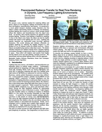
Precomputed Radiance Transfer for Real-Time Renderingin Dynamic, Low-Frequency Lighting EnvironmentsPeter-Pike SloanJan KautzJohn SnyderMicrosoft ResearchMax-Planck-Institut für InformatikMicrosoft johnsny@microsoft.comAbstractWe present a new, real-time method for rendering diffuse andglossy objects in low-frequency lighting environments that captures soft shadows, interreflections, and caustics. As a preprocess,a novel global transport simulator creates functions over theobject’s surface representing transfer of arbitrary, low-frequencyincident lighting into transferred radiance which includes globaleffects like shadows and interreflections from the object ontoitself. At run-time, these transfer functions are applied to actualincident lighting. Dynamic, local lighting is handled by samplingit close to the object every frame; the object can also be rigidlyrotated with respect to the lighting and vice versa. Lighting andtransfer functions are represented using low-order sphericalharmonics. This avoids aliasing and evaluates efficiently ongraphics hardware by reducing the shading integral to a dotproduct of 9 to 25 element vectors for diffuse receivers. Glossyobjects are handled using matrices rather than vectors. We furtherintroduce functions for radiance transfer from a dynamic lightingenvironment through a preprocessed object to neighboring pointsin space. These allow soft shadows and caustics from rigidlymoving objects to be cast onto arbitrary, dynamic receivers. Wedemonstrate real-time global lighting effects with this approach.Keywords: Graphics Hardware, Illumination, Monte Carlo Techniques,Rendering, Shadow Algorithms.1. IntroductionLighting from area sources, soft shadows, and interreflections areimportant effects in realistic image synthesis. Unfortunately,general methods for integrating over large-scale lighting environments [8], including Monte Carlo ray tracing [7][21][25], radiosity [6], or multi-pass rendering that sums over multiple pointlight sources [17][27][36], are impractical for real-time rendering.Real-time, realistic global illumination encounters three difficulties – it must model the complex, spatially-varying BRDFs of realmaterials (BRDF complexity), it requires integration over thehemisphere of lighting directions at each point (light integration),and it must account for bouncing/occlusion effects, like shadows,due to intervening matter along light paths from sources to receivers (light transport complexity). Much research has focused onextending BRDF complexity (e.g., glossy and anisotropic reflections), solving the light integration problem by representingincident lighting as a sum of directions or points. Light integration thus tractably reduces to sampling an analytic or tabulatedBRDF at a few points, but becomes intractable for large lightsources. A second line of research samples radiance and preconvolves it with kernels of various sizes [5][14][19][24][34].This solves the light integration problem but ignores light transport complexities like shadows since the convolution assumes theincident radiance is unoccluded and unscattered. Finally, clevertechniques exist to simulate more complex light transport, especially shadows. Light integration becomes the problem; thesetechniques are impractical for very large light sources.Our goal is to better account for light integration and light transport complexity in real-time. Our compromise is to focus on low-Figure 1: Precomputed, unshadowed irradiance from [34] (left) vs. ourprecomputed transfer (right). The right model can be rendered at 129Hzwith self-shadowing and self-interreflection in any lighting environment.frequency lighting environments, using a low-order sphericalharmonic (SH) basis to represent such environments efficientlywithout aliasing. The main idea is to represent how an objectscatters this light onto itself or its neighboring space.To describe our technique, assume initially we have a convex,diffuse object lit by an infinitely distant environment map. Theobject’s shaded “response” to its environment can be viewed as atransfer function, mapping incoming to outgoing radiance, whichin this case simply performs a cosine-weighted integral. A morecomplex integral captures how a concave object shadows itself,where the integrand is multiplied by an additional transport factorrepresenting visibility along each direction.Our approach is to precompute for a given object the expensivetransport simulation required by complex transfer functions likeshadowing. The resulting transfer functions are represented as adense set of vectors or matrices over its surface. Meanwhile,incident radiance need not be precomputed. The graphics hardware can dynamically sample incident radiance at a number ofpoints. Analytic models, such as skylight models [33] or simplegeometries like circles, can also be used.By representing both incident radiance and transfer functions in alinear basis (in our case, SH), we exploit the linearity of lighttransport to reduce the light integral to a simple dot productbetween their coefficient vectors (diffuse receivers) or a simplelinear transform of the lighting coefficient vector through a smalltransfer matrix (glossy receivers). Low-frequency lighting environments require few coefficients (9-25), enabling graphicshardware to compute the result in a single pass (Figure 1, right).Unlike Monte-Carlo and multi-pass light integration methods, ourrun-time computation stays constant no matter how many or howbig the light sources, and in fact relies on large-scale, smoothlighting to limit the number of SH coefficients necessary.We represent complex transport effects like interreflections andcaustics in the transfer function. Since these are simulated as apreprocess, only the transfer function’s basis coefficients areaffected, not the run-time computation. Our approach handlesboth surface and volume-based geometry. With more SH coefficients, we can even handle glossy (but not highly specular)receivers as well as diffuse, including interreflection. 25 coefficients suffice for useful glossy effects. In addition to transferfrom a rigid object to itself, called self-transfer, we generalize thetechnique to neighborhood-transfer from a rigid object to itsneighboring space, allowing cast soft shadows, glossy reflections,and caustics on dynamic receivers, see Figure 7.
Overview As a preprocess, a global illuminationsimulator is run over the model that captures how itshadows and scatters light onto itself. The result isrecorded as a dense set of vectors (diffuse case) ormatrices (glossy case) over the model. At run-time(Figure 2), incident radiance is first projected to the SHbasis. The model’s field of transfer vectors or matricesis then applied to the lighting’s coefficient vector. If theobject is diffuse, a transfer vector at each point on theobject is dotted with the lighting’s coefficients toproduce correctly self-scattered shading. If the object isglossy, a transfer matrix is applied to the lightingcoefficients to produce the coefficients of a sphericalfunction representing self-scattered incident radiance ateach point. This function is convolved with the object’sBRDF and then evaluated at the view-dependent reflection direction to produce the final shading.diffuse surface self-transfer2. Related WorkScene relighting precomputes a separate global illumination solution per light source as we do; linearcombinations of the results then provide limited dynamic effects. Early work [2][11] adjusts intensities ofa fixed set of sources and is not intended to fit generallighting environments. Nimeroff, et al. [33] precomputea “steerable function” basis for general skylight illumination on a fixed view. Their basis, essentially theglossy surface self-transferspherical monomials, is related to the SH by a lineartransformation and thus shares some of its propertiesFigure 2: Self-Transfer Run-Time Overview. Red signifies positive SH coefficients(e.g., rotational invariance) but not others (e.g., orand blue, negative. For a diffuse surface (top row), the SH lighting coefficients (on thethonormality). Teo, et al. [40] generalize to non-infiniteleft) modulate a field of transfer vectors over the surface (middle) to produce the finalresult (right). A transfer vector at a particular point on the surface represents how thesources, using principal component analysis to reducesurface responds to incident light at that point, including global transport effects likethe basis set. Our work differs by computing a transferself-shadowing and self-interreflection. For a glossy surface (bottom row), there is afield over the object’s surface in 3D rather than over amatrix at each point on the model instead of a vector. This matrix transforms the lightfixed 2D view to allow viewpoint changes. Dobashi, eting coefficients into the coefficients of a spherical function representing transferredal. [10] use the SH basis and transfer vector fields overradiance. The result is convolved with the model’s BRDF kernel and evaluated at thesurfaces to allow viewpoint change but restrict lightingview-dependent reflection direction R to yield the result at one point on the model.changes to the directional intensity distribution of aninterreflection change due to dynamic lighting is still not realexisting set of non-area light sources in diffuse scenes. Debevec,time. By precomputing a higher-dimensional texture, polynomialet al. [9] relight faces using a directional light basis. Real-timetexture maps [30] allow real-time interreflection effects as well asrendering requires a fixed view.shadowing. A similar approach using a steerable basis for direcShadow maps, containing depths from the light source’s point oftional lighting is used in [3]. Like our approach, these methodsview, were first used by Williams [43] to simulate point lightprecompute a simple representation of a transfer function, but onesource shadows. Many extensions of the basic technique, somebased on directional light sources and thus requiring costly multisuitable for real-time rendering, have since been described:pass integration to simulate area lights. We compute self-transferpercentage-closer filtering [35], which softens shadow edges,directly on each preprocessed 3D object rather than mapping itlayered depth maps [26] and layered attenuation maps [1], whichwith 2D micro-geometry textures, allowing more global effects.more accurately simulate penumbra shape and falloff, and deepFinally, our neighborhood transfer extends these ideas to castshadow maps [29], which generalize the technique to partiallyshadows, caustics, and reflections.transparent and volume geometry. All these techniques assumeCaching onto diffuse receivers is useful for accelerating globalpoint or at least localized light sources; shadowing from largerillumination. Ward et. al. [41] perform caching to simulatelight sources has been handled by multi-pass rendering that sumsdiffuse interreflection in a ray tracer. Photon maps [21] alsoover a light source decomposition into points or small sourcescache but perform forward ray tracing from light sources rather[17][27][36]. Large light sources become very expensive.than backwards from the eye, and handle specular bounces in theAnother technique [39] uses FFT convolution of occluder projectransport (as does our approach). We apply this caching idea totions for soft shadowing with cost independent of light sourcereal-time rendering, but cache a transfer function parameterizedsize. Only shadows between pre-segmented clusters of objectsby a SH lighting basis rather than scalar irradiance.are handled, making self-shadows on complex meshes difficult.Precomputed transfer using light-field remapping [18] andFinally, accessibility shading [32] is also based on precomputeddynamicray tracing [16] has been used to achieve highly specularglobal visibility, but is a scalar quantity that ignores changes inreflections and refractions. We apply a similar precomputed, perlighting direction.object decomposition but designed instead for soft shadows andMethods for nonlocal lighting on micro-geometry include thecaustics on nearly diffuse objects in low-frequency lighting.horizon map [4][31], which efficiently renders self-shadowingIrradiance volumes [15] allow movement of diffuse receivers infrom point lights. In [20], this technique is tailored to graphicsprecomputed lighting. Unlike our approach, lighting is static andhardware and generalized to diffuse interreflections, thoughthe receiver’s effect on itself and its environment is ignored.
Spherical harmonics have been used to represent incident radiance and BRDFs for offline rendering and BRDF inference [4][38][42]. Westin, et al. [42] use a matrix representation for 4DBRDF functions in terms of the SH basis identical to our transfermatrix. But rather than the BRDF, we use it to represent globaland spatially varying transport effects like shadows. The SH basishas also been used to solve ambiguity problems in computervision [12] and to represent irradiance for rendering [34].3. Review of Spherical HarmonicsDefinition Spherical harmonics define an orthonormal basis overthe sphere, S, analogous to the Fourier transform over the 1Dcircle. Using the parameterizations ( x, y, z ) (sin q cos j , sinq sin j , cosq ) ,the basis functions are defined asYl m (q ,j ) K lm eimj Pl m (cosq ), l Œ N , -l m lwhere Plm are the associated Legendre polynomials and Klm arethe normalization constantsK lm (2l 1) (l - m )!.4p (l m )!The above definition forms a complex basis; a real-valued basis isgiven by the simple transformationÏ 2 Re(Yl m ), m 0 Ï 2 K lm cos(mj ) Pl m (cosq ), m 0ÔÔÔÔylm Ì 2 Im(Yl m ), m 0 Ì 2 K lm sin( - mj ) Pl - m (cosq ), m 0ÔY 0 ,m 0 Ô Kl0 Pl 0 (cosq ),m 0ÓÔ lÓÔLow values of l (called the band index) represent low-frequencybasis functions over the sphere. The basis functions for band lreduce to polynomials of order l in x, y, and z. Evaluation can bedone with simple recurrence formulas [13][44].Projection and Reconstruction Because the SH basis is orthonormal, a scalar function f defined over S can be projectedinto its coefficients via the integralf l m Ú f ( s ) ylm ( s) ds(1)These coefficients provide the n-th order reconstruction functionn -1f ( s ) ÂlÂl 0 m -lfl m ylm ( s )(2)which approximates f increasingly well as the number of bands nincreases. Low-frequency signals can be accurately representedwith only a few SH bands. Higher frequency signals are bandlimited (i.e., smoothed without aliasing) with a low-order projection.Projection to n-th order involves n2 coefficients. It is often convenient to rewrite (2) in terms of a singly-indexed vector ofprojection coefficients and basis functions, vian2f ( s )  fi yi ( s)(3)i 1where i l(l 1) m 1. This formulation makes it obvious thatevaluation at s of the reconstruction function represents a simpledot product of the n2-component coefficient vector fi with thevector of evaluated basis functions yi(s).Basic Properties A critical property of SH projection is itsrotational invariance; that is, given g ( s ) f (Q( s )) where Q is anarbitrary rotation over S theng ( s ) f (Q( s ))(4)This is analogous to the shift-invariance property of the 1DFourier transform. Practically, this property means that SHprojection causes no aliasing artifacts when samples from f arecollected at a rotated set of sample points.Orthonormality of the SH basis provides the useful property thatgiven any two functions a and b over S, their projections satisfyn2Ú a (s) b (s) ds  ai bi .(5)i 1In other words, integration of the product of bandlimited functionsreduces to a dot product of their projection coefficients.Convolution We denote convolution of a circularly symmetrickernel function h(z) with a function f as h * f . Note that h mustbe circularly symmetric (and hence can be defined as a simplefunction of z rather than s) in order for the result to be defined onS rather than the higher-dimensional rotation group SO(3).Projection of the convolution satisfies4p(6)hl0 f l m a l0 hl0 fl m .2l 1In other words, the coefficients of the projected convolution aresimply scaled products of the separately projected functions.Note that because h is circularly symmetric about z, its projectioncoefficients are nonzero only for m 0. The convolution propertyprovides a fast way to convolve an environment map with ahemispherical cosine kernel, defined as h( z ) max( z ,0) , to getan irradiance map [34], for which the hl0 are given by an analyticformula. The convolution property can also be used to produceprefiltered environment maps with narrower kernels.Product Projection Projection of the product of a pair of spherical functions c( s) a( s ) b( s) where a is known and b unknowncan be viewed as a linear transformation of the projection coefficients bj via a matrix â :(h * f )lm ()ci Ú a( s ) b j y j ( s ) yi ( s ) ds (Ú a(s) y (s) y (s) ds) b (a Ú y (s) y (s) y (s) ds) b aˆ bijjkijkjij(7)jwhere summation is implied over the duplicated j and k indices.Note that â is a symmetric matrix. The components of â can becomputed by integrating the triple product of basis functions usingrecurrences derived from the well-known Clebsch-Gordan series[13][44]. It can also be computed using numerical integrationwithout SH-projecting the function a beforehand. Note that theproduct’s order n projection involves coefficients of the two factorfunctions up to order 2n-1.Rotation A reconstruction function rotated by Q, f (Q( s )) , canbe projected into SH using a linear transformation of f’s projection coefficients, fi. Because of the rotation invariance property,this linear transformation treats the coefficients in each bandindependently. The most efficient implementation is achieved viaa zyz Euler angle decomposition of the rotation Q, using a fairlycomplicated recurrence formula [13][44]. Because we deal onlywith low-order functions, we have implemented their explicitrotation formulas using symbolic integration.4. Radiance Self-TransferRadiance self-transfer encapsulates how an object O shadows andscatters light onto itself. To represent it, we first parameterizeincident lighting at points p ŒO , denoted Lp(s), using the SHbasis. Incident lighting is therefore represented as a vector of n2coefficients (Lp)i. We sample the lighting dynamically andsparsely near the surface, perhaps at only a single point. Theassumption is that lighting variation over O not due to its ownpresence is small (see Section 6.1). We also precompute andstore densely over O transfer vectors or matrices.A transfer vector (Mp)i is useful for diffuse surfaces and represents a linear transformation on the lighting vector producingscalar exit radiance, denoted L p , via the inner productn2Lp  ( M p )i ( L p )ii 1.(8)
be inaccurate even for smooth lighting environments since Vp cancreate higher-frequency lighting locally, e.g., by self-shadowing“pinholes”. 4-th or 5-th order projection provides good results ontypical meshes in smooth lighting environments.Finally, to capture diffuse interreflections as well as shadows, wedefine interreflected diffuse transfer as(TDI ( Lp ) TDS ( L p ) r p p(a) unshadowed(b) shadowed(c) interreflectedFigure 3: Diffuse Surface Self-transfer.In other words, each component of (Mp)i represents the linearinfluence that a lighting basis function (Lp)i has on shading at p.A transfer matrix (Mp )ij is useful for glossy surfaces and represents a linear transformation on the lighting vector whichproduces projection coefficients for an entire spherical function oftransferred radiance Lp ( s ) rather than a scalar; i.e.,n2( Lp )i  (Mp )ij ( L p ) j .(9)j 1The difference between incident and transferred radiance is thatLp ( s ) includes shadowing/scattering effects due to the presenceof O while Lp(s) represents incident lighting assuming O wasremoved from the scene. Components of (Mp )ij represent thelinear influence of the j-th lighting coefficient of incident radiance(Lp)j to the i-th coefficient of transferred radiance ( L p )i . The nextsections derive transfer vectors for diffuse surfaces and transfermatrixes for glossy surfaces due to self-scattering on O.4.1 Diffuse Transfer [transfer vector for known normal]First assume O is diffuse. The simplest transfer function at apoint p ŒO represents unshadowed diffuse transfer, defined as thescalar function(TDU ( L p ) r p p) Ú L (s) HpNp( s ) dsproducing exit radiance which is invariant with view angle fordiffuse surfaces. Here, r p is the object’s albedo at p, Lp is theincident radiance at p assuming O was removed from the scene,Np is the object’s normal at p, and H Np ( s) max( N p i s,0) is theBy SHcosine-weighted, hemispherical kernel about Np.projecting Lp and HNp separately, equation (5) reduces TDU to aninner product of their coefficient vectors. We call the resultingfactors the light function, Lp, and transfer function, Mp. In thisfirst simple case, M pDU ( s ) H Np ( s ) .Because Np is known, the SH-projection of the transfer function( M pDU )i can be precomputed, resulting in a transfer vector. Infact, storing is unnecessary because a simple analytic formulayields it given Np. Because M pDU is inherently a low-pass filter,second-order projection (9 coefficients) provides good accuracy inan arbitrary (even non-smooth) lighting environment [34].To include shadows, we define shadowed diffuse transfer as(TDS ( Lp ) r p p) Ú L (s) HpNp( s )V p ( s ) dswhere the additional visibility function, V p ( s ) Æ {0,1} , equals 1when a ray from p in the direction s fails to intersect O again (i.e.,is unshadowed). As with unshadowed transfer, we decomposethis integral into two functions, using an SH-projection of Lp andthe transfer functionM pDS ( s ) H Np ( s)V p ( s) .(10)Separately SH-projecting Lp and Mp againreduces the integral in TDS to an innerproduct of coefficient vectors.Transfer is now nontrivial; we precomputeit using a transport simulator (Section 5),storing the resulting transfer vector (Mp)i atmany points p over O. Unlike the previouscase, second-order projection of M pDS may(a) unshadowed) Ú L ( s) HpNp()()( s ) 1 - V p ( s ) dswhere Lp ( s ) is the radiance from O itself in the direction s. Thedifficulty is that unless the incident radiance emanates from aninfinitely-distant source, we don’t actually know Lp ( s ) given theincident radiance only at p because Lp depends on the exitradiance of points arbitrarily far from p and local lighting variesover O. If lighting variation is small over O then Lp is wellapproximated as if O were everywhere illuminated by Lp. TDIthus depends linearly on Lp and can be factored as in the previoustwo cases into a product of two projected functions: one lightdependent and the other geometry-dependent.Though precomputed interreflections must make the assumptionof spatially invariant incident lighting over O, simpler shadowedtransfer need not. The difference is that shadowed transfer depends only on incident lighting at p, while interreflected transferdepends on many points q π p over O at which Lq π L p . Thus,as long as the incident radiance field is sampled finely enough(Section 6.1), local lighting variation can be captured and shadowed transfer will be correct.The presence of L makes it hard to explicitly denote the transferfunction for interreflections, M pDI ( s ) . We will see how to compute its projection coefficients numerically in Section 5.4.2 Glossy Transfer [transfer matrix for unknown direction]Self-transfer for glossy objects can be defined similarly, butgeneralizes the kernel function to depend on a (view-dependent)reflection direction R rather than a (fixed) normal N. Analogousto the H kernel from before, we model glossy reflection as thekernel G(s,R,r) where a scalar r defines the “glossiness” or broadness of the specular response. We believe it is possible to handlearbitrary BRDFs as well using their SH projection coefficients[38] but this remains for future work.We can then define the analogous three glossy transfer functionsfor the unshadowed, shadowed, and interreflected cases asTGU ( Lp , R, r ) Ú Lp ( s ) G ( s, R, r ) dsTGS ( L p , R, r ) Ú Lp ( s ) G ( s, R, r )V p ( s ) dsTGI ( Lp , R, r ) TGS ( Lp ) Ú Lp ( s ) G ( s, R, r ) 1 - V p ( s ) dswhich output scalar radiance in direction R as a function of Lp andR, quantities both unknown at precomputation time. Since transfer is no longer solely a function of s, it can’t be reduced to asimple vector of SH coefficientsInstead of parameterizing scalar transfer by R and r, a more usefuldecomposition is to transfer the incident radiance Lp(s) into awhole sphere of transferred radiance, denoted Lp ( s ) . Assumingthe glossy kernel G is circularly symmetric about R (i.e., a simplePhong-like model) Lp ( s ) can then be convolved withGr* ( z ) G ( s,(0,0,1), r ) and evaluated at R to produce the final(b) shadowedFigure 4: Glossy Surface Self-transfer.(c) interreflected
result (see bottom of Figure 2, and further details in Section 6).Transfer to L p can now be represented as a matrix rather than avector. For example, glossy shadowed transfer isMpGS ( Lp , s ) Lp ( s )V p ( s )(11)a linear operator on Lp whose SH-projection can be represented asthe symmetric matrix Vˆp via equation (7). Even with smoothlighting, more SH bands must be used for L p as O’s glossinessincreases; non-square matrices (e.g., 25 9) mapping lowfrequency lighting to higher-frequency transferred radiance areuseful under these conditions. For shadowed glossy transfer (butnot interreflected), an alternative still uses a vector rather than amatrix to represent MpGS by computing the product of Vp with Lpon-the-fly using the tabulated triple product of basis functions inequation (7). We have not yet implemented this alternative.4.3 Limitations and DiscussionAn important limitation of precomputed transfer is that materialproperties of O influencing interreflections in TDI and TGI (likealbedo or glossiness) must be “baked in” to the preprocessedtransfer and can’t be changed at run-time. On the other hand, thesimpler shadowed transfer without interreflection does allow runtime change and/or spatial variation over O of the material properties. Error arises if blockers or light sources intrude into O’sconvex hull. O can only move rigidly, not deform or move onecomponent relative to the whole. Recall also the assumption oflow lighting variation over O required for correct interreflections.Finally, note that diffuse transfer as defined produces radianceafter leaving the surface, since it has already been convolved withthe cosine-weighted normal hemisphere, while glossy transferproduces radiance incident on the surface and must be convolvedwith the local BRDF to produce the final exit radiance. It’s alsopossible to bake in a fixed BRDF for glossy O, making the convolution with G unnecessary at run-time but limiting flexibility.5. Precomputing Radiance Self-TransferAs a preprocess, we perform a global illumination simulation overan object O using the SH basis over the infinite sphere as emitters.Our light gathering solution technique is a straightforward adaptation of existing approaches [7][25] and could be accelerated inmany ways; its novelty lies in how it parameterizes the lightingand collects the resulting integrated transfers. Note that allintegrated transfer coefficients are signed quantities.The simulation is parameterized by an n-th order SH projection ofthe unknown sphere of incident light L; i.e., by n2 unknowncoefficients Li. Though the simulation results can be computedindependently for each Li using the SH basis function yi(s) as anemitter, it is more efficient to compute them all at once. Theinfinitely-distant sphere L will be replaced at run-time by theactual incident radiance field around O, Lp.An initial pass simulates direct shadows from paths leaving L andreaching sample points p ŒO . In subsequent passes, interreflections are added, representing paths from L that bounce a numberof times off O before arriving at p (Lp, LDp, LDDp, etc.). In eachpass, energy is gathered to every sample point p. Large emitters(i.e., low-frequency SH basis) make a gather more efficient then ashooting-style update [6]. Note that this idea of caching ontodiffuse (or nearly diffuse) receivers is not new [21][41].To capture the sphere of directions at sample points p ŒO , wegenerate a large (10k-30k), quasi-random set of directions {sd},sd Œ S . We also precompute evaluations for all the SH basisfunctions at each sd. The sd are organized in hierarchical binsformed by refining an initial icosahedron with 1 2 bisection intoequal-area spherical triangles (1 4 subdivision does not lead toequal area triangles on the sphere as it does in the plane). We use6 to 8 subdivision levels, creating 512 to 2048 bins. Every bin ateach level of the hierarchy contains a list of the sd within it.In the first pass, for each p ŒO , we cast shadow rays in thehemisphere about p’s normal Np, using the hierarchy to culldirections outside the hemisphere. We tag each direction sd withan occlusion bit, 1 - V p ( sd ) , indicating whether sd is in the hemisphere and intersects O again (i.e., is self-shadowed by O). Anocclusion bit is also associated with the hierarchical bins, indicating whether any sd within it is occluded. Self-occluded directionsand bins are tagged so that we can perform further interreflectionpasses on them; completely unoccluded bins/samples receive onlydirect light from the environment.For diffuse surfaces, at each point p ŒO we further compute thetransfer vector by SH-projecting Mp from (10). For glossy surfaces, we compute the transfer matrix by SH-projecting Mp from(11). In either case, the result represents the radiance collected atp, parameterized by L. SH-projection to compute the transfers isperformed b
real-time rendering, but cache a transfer function parameterized by a SH lighting basis rather than scalar irradiance. Precomputed transfer using light-field remapping [18] and dynamic ray tracing [16] has been used to achieve highly specular reflecti