Transcription
End-to-End SMT with Zero or Small Parallel Texts1AbstractWe use bilingual lexicon induction techniques, which learn translations from monolingual texts in two languages, to build an end-to-end statistical machine translation (SMT)system without the use of any bilingual sentence-aligned parallel corpora. We presentdetailed analysis of the accuracy of bilingual lexicon induction, and show how a discriminative model can be used to combine various signals of translation equivalence (like contextual similarity, temporal similarity, orthographic similarity and topic similarity). Ourdiscriminative model produces higher accuracy translations than previous bilingual lexicon induction techniques. We reuse these signals of translation equivalence as features on aphrase-based SMT system. These monolingually-estimated features enhance low resourceSMT systems in addition to allowing end-to-end machine translation without parallelcorpora.
Natural Language Engineering 1 (1): 1–34.Printed in the United Kingdom2c 2015 Cambridge University PressEnd-to-End Statistical Machine Translation withZero or Small Parallel TextsAnn Irvine and Chris Callison-Burch( Received December 15, 2014 )1 IntroductionSMT typically relies on very large amounts of bilingual sentence-aligned paralleltexts. Here, we consider settings in which we have access to (1) bilingual dictionariesbut no parallel sentences for training, and (2) only a small amount of paralleltraining data. In the first case, we augment a baseline system that produces a simpledictionary gloss with additional translations that are learned using monolingualcorpora in the source and target languages. In the second case, we wish to augmenta baseline statistical model learned over small amounts of parallel training datawith additional translations and features estimated over monolingual corpora.In this article, we detail our approach to bilingual lexicon induction, which allowsus to learn translations from independent monolingual texts or comparable corporathat are written in two languages (Section 2). We evaluate the accuracy of ourmodel on correctly learning dictionary translations, and examine its performanceon low frequency words which are more likely to be out of vocabulary (OOV) withrespect to the training data for SMT systems.We describe our approach to learning how to transliteration from one language’sscript into another language’s script (Section 3). Transliteration is a useful aid,since many OOV items correspond to named entities or technical terms, which areoften transliterated rather than translated.We show how the diverse signals of translation equivalence that we use in ourdiscriminative model for bilingual lexicon induction can also be used as additionalfeatures for a phrase table in a standard SMT model to enhance low resourceSMT systems (Section 4). We analyze 6 low resource languages and find consistentimprovements in BLEU score when we incorporate translations of OOV items andwhen we re-score the phrase table with additional monolingually estimated featurefunctions.Finally, we combine all of these ideas and demonstrate how to build a true end-toend SMT system without bilingual sentence-aligned parallel corpora (Section 5). Webuild a patchwork phrase table out of entries from a standard bilingual dictionaries,plus induced translations, plus transliterations. We associate each translation witha set of monolingually-estimated feature functions and generate translations usinga SMT decoder that incorporates these scores and a language model probability.This article combines and extends several of our past papers on this topic: (Irvine,
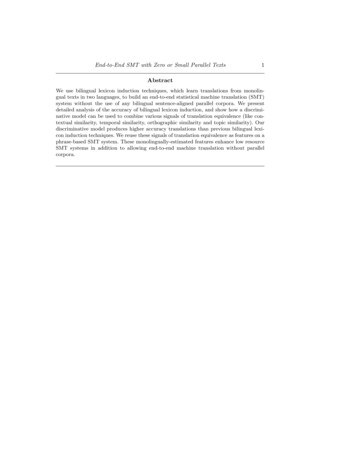
End-to-End SMT with Zero or Small Parallel Texts100100% Word Tokens OOV80 TamilTeluguBengaliHindi 80% Word Types OOV 603 40 60 40 20 TamilTeluguBengaliHindi20 005e 031e 042e 045e 04Words of Training Data(a) Tokens1e 052e 055e 031e 042e 045e 041e 052e 05Words of Training Data(b) TypesFig. 1: The rate of out of vocabulary (OOV) items for six low resources languages.We show the token-based and type-based OOV rates. The curves are generated byrandomly sampling the training datasets described in Section 4.1.Callison-Burch, and Klementiev2010), (Irvine and Callison-Burch2013b), (Irvineand Callison-Burch2013a), (Irvine2014) and (Irvine and Callison-BurchIn submission). This article expands the previous publications by providing additional analysis and examples from Ann Irvine’s PhD thesis. The main experimental resultsthat were not previously published are the expanded set of experiments on our discriminative model for bilingual lexicon induction (Section 2). Because this articleassembles research undertaken over a period of 5 years, it is not perfectly consistent from section to section in terms of what languages it analyzes or in usingidentical features across all experiments. Despite this, we believe that this articleprovides a valuable synthesis of our past work on trying to improve SMT for lowresource languages, with the aim of reducing or eliminating the dependency onsentence-aligned bilingual parallel corpora.2 Learning Translations of Unseen WordsSMT typically uses sentence-aligned bilingual parallel texts to learn the translationsof individual words (Brown et al.1990). Another thread of research has examinedbilingual lexicon induction which tries to induce translations from monolingual corpora in two languages. These monolingual corpora can range from being completelyunrelated topics to being comparable corpora. Here we examine the usefulness ofbilingual lexicon induction as a way of augmenting SMT when we only have accessto small bilingual parallel corpora, and when we have no bitexts whatsoever.The most prominent problem that arises when a machine translation system hasaccess to limited parallel resources is the fact that there are many unknown words
4Irvine and Callison-Burchthat are OOV with respect to the training data, but which do appear in the textsthat we would like the SMT system to translate. Figure 1 quantifies the rate ofOOVs for half a dozen low resource languages. It shows the percent of word tokensand word types in a development set that are OOV with respect to varying amountsof training data for several Indian languages.1 Bilingual lexicon induction can beused to try to improve the coverage of our low resource translation models, bylearning the translations of words that do not occur in the parallel training data.Although past research into bilingual lexicon induction has been motivated bythe idea that it could be used to improve machine translation systems by translating OOV words, it has rarely been evaluated that way. Notable exceptions of pastresearch that does evaluate bilingual lexicon induction in the context of machinetranslation through better OOV handling include (Daumé and Jagarlamudi2011),(Dou and Knight2013) and (Dou, Vaswani, and Knight2014). However, the majority of prior work in bilingual lexicon induction has treated it as a standalone task,without actually integrating induced translations into end-to-end machine translation. It was instead evaluated by holding out a portion of a bilingual dictionary andevaluating how well the algorithm learns the translations of the held out words. Inthis article, we perform a systematic examination of the efficacy of bilingual lexiconinduction for end-to-end translation.Bilingual lexicon induction uses monolingual or comparable corpora, usuallypaired with a small seed dictionary, to compute signals of translation equivalence.Here we briefly describe our approach to bilingual lexicon induction that combinesmultiple signals of translation equivalence in a discriminative model. More detailsabout our approach are available in (Irvine and Callison-Burch2013b), (Irvine2014),and (Irvine and Callison-BurchIn submission). Although past research into bilingual lexicon induction also explored multiple signals of translation equivalence (forinstance, (Schafer and Yarowsky2002)), these features have not previously beencombined using a discriminative model.2.1 Our approach to bilingual lexicon inductionWe frame bilingual lexicon induction as a binary classification problem: for a pairof source and target language words, we predict whether the two are translations ofone another or not. Since binary classification does not inherently give us a list of thebest translations, we need to take an additional step. For a given source languageword we find its best translation or its n-best translations by first using our classifieron all target language words. We then rank them based on how confident theclassifier is that each target word is a translation of the source word. The featuresused by our classifier include a variety of signals of translation equivalence thatare drawn from past work in bilingual lexicon induction, notably by (Rapp1995;1Our Indian language datasets are described in Section 4.1. Note that in this OOVanalysis, we do not include the dictionaries, only complete sentences of bilingual trainingdata.
End-to-End SMT with Zero or Small Parallel Textsrápidamente 7planetaeconomías eo vityexpandFig. 2: Example of projecting contextual vectors over a seed bilingual lexicon. TheSpanish word crecer appears in the context of the words empleo, extranjero, etc inmonolingual texts. We use this co-occurence information to build a context vector.Each position in the context vector for corresponds to a word in the Spanish vocabulary. The vector for crecer is projected into the English vector space using asmall seed dictionary. Context vectors for all English words (policy, expand, etc.)are collected and then compared against the projected context vector for Spanishcrecer. Finally, contextual similarities are calculated by comparing the projectedvector with the context vector of each target word using cosine similarity. Wordpairs with high cosine similarity are likely to be translations of one another.Fung1995; Schafer and Yarowsky2002; Klementiev and Roth2006; Klementiev etal.2012), and others. The features that we use in our model are: Contextual similarity – In a similar fashion to how vector space modelscan be used to compute the similarity between two words in one languageby creating vectors that representing their co-occurrence patterns with otherwords (Turney and Pantel2010), context vector representations can also beused to compare the similarity of words across two languages. The earliestwork in bilingual lexicon induction by (Rapp1995) and (Fung1995) used thesurrounding context of a given word as a clue to its translation. (Fung andYee1998) and (Rapp1999), used small seed dictionaries to project word-basedcontext vectors from the vector space of one language into the vector spaceof the other language. We use the vector space approach of (Rapp1999) tocompute similarity between word in the source and target languages.More formally, assume that (s1 , s2 , . . . sN ) and (t1 , t2 , . . . tM ) are (arbitrarilyindexed) source and target vocabularies, respectively. A source word f isrepresented with an N -dimensional vector and a target word e is representedwith an M -dimensional vector (see Figure 2). The component values of thevector representing a word correspond to how often each of the words in thatvocabulary appear within a two word window on either side of the given word.These counts are collected using monolingual corpora. After the values have
6Irvine and Callison-Burchbeen computed, a contextual vector for f is projected onto the English vectorspace using translations in a given bilingual dictionary to map the componentvalues into their appropriate English vector positions. This sparse projectedvector is compared to the vectors representing all English words, e. Each wordpair is assigned a contextual similarity score based on the similarity betweene and the projection of f .Various means of computing the component values and vector similarity measures have been proposed in literature (e.g. (Fung and Yee1998; Rapp1999)).Following (Fung and Yee1998), we compute the value of the k-th componentof f ’s contextual vector, fk , as follows:(1)fk nf,k (log(n/nk ) 1)where nf,k and nk are the number of times sk appears in the context of fand in the entire corpus, and n is the maximum number of occurrences of anyword in the data. Intuitively, the more frequently sk appears with fi and theless common it is in the corpus in general, the higher its component value.After projecting each component of the source language contextual vectorsinto the English vector space, we are left with M -dimensional source wordcontextual vectors, Fcontext , and correspondingly ordered M -dimensional target word contextual vectors, Econtext , for all words in the vocabulary of eachlanguage. We use cosine similarity to measure the similarity between eachpair of contextual vectors:(2)simcontext (Fcontext , Econtext ) Fcontext · Econtext Fcontext Econtext Temporal similarity – Usage of words over time may be another signal oftranslation equivalence. The intuition that is that news stories in differentlanguages will tend to discuss the same world events on the same day and,correspondingly, we expect that source and target language words which aretranslations of one another will appear with similar frequencies over timein monolingual data. For instance, if the English word tsunami is used frequently during a particular time span, the Spanish translation maremoto islikely to also be used frequently during that time. To calculate temporal similarity, we collected online monolingual newswire over a multi-year periodand associate each article with a time stamps. We gather temporal signatures for each source and target language unigram from our time-stampedweb crawl data in order to measure temporal similarity, in a similar fashionto (Schafer and Yarowsky2002; Klementiev and Roth2006; Alfonseca, Ciaramita, and Hall2009). We calculate the temporal similarity between a pairof words, using the method defined by (Klementiev and Roth2006). Orthographic similarity – Words that are spelled similarly are sometimesgood translations, since they may be etymologically related, or borrowedwords, or the names of people and places. We compute the orthographic
End-to-End SMT with Zero or Small Parallel Texts7Wikipedia15Barack ObamaОбама, Барак81032VirginiaВиргиния150210Iraq WarИракская война8000ÜckeritzИккериц0001Otto von BismarckБисмарк, Отто окtroopsвойскаFig. 3: Illustration of how we compute the topical similarity between troops andthree Russian candidate translations. We first collect the topical signatures foreach word (e.g. troops appears in the page about Barack Obama 15 times and inthe page about Virginia 32 times.) based on the interlingually linked pages. We canthen directly compare each pair of topical signatures.similarity between a pair of words using Levenshtein edit distance2 , normalized by the average of the lengths of the two words. This is straightforwardfor languages which use the same character set, but it is more complicatedfor languages that are written using different scripts. For non-Roman scriptlanguages, we transliterate words into the Roman script before measuringorthographic similarity with their candidate English translations (Virga andKhudanpur2003; Irvine, Callison-Burch, and Klementiev2010). More detailsof our transliteration method are given in Section 3. Topic similarity – Articles that are written about the same topic in twolanguages, are likely to contain words and their translations, even if the articles themselves are written independently and are not translations of oneanother. We use Wikipedia’s interlingual links to identify comparable articlesacross languages. These links define a number of topics, and we construct atopic vector. We compute cosine distance between topic signatures.(3)simtopic (Ftopic , Etopic ) Ftopic · Etopic, Ftopic Etopic The length of a word’s topic vector is the number of interlingually linkedarticle pairs. Each component fk of Ftopic is the count of the word f inthe foreign article from the kth linked article pair, normalized by the totaloccurrences of k. The dimensionality of the topic signatures varies dependingon the language pair. The number of linked articles in Wikipedia range from84 (between Kashmiri and English) to over 500 thousand (between French andEnglish). Figure 3 illustrates this signal. More details on our topic similarityare in tein distance
8Irvine and Callison-Burch Frequency similarity – Words that are translations of one another arelikely to have similar relative frequencies in monolingual corpora. We measurethe frequency similarity of two words, simf req , as the absolute value of thedifference between the log of their relative corpus frequencies, or:(4)f req(e)f req(f )simf req (e, f ) log( P) log( P) freq(e)iii f req(fi )This helps prevent high frequency closed class words from being consideredviable translations of less frequent open class words. Burstiness similarity – Burstiness is a measure of how peaked a word’susage is over a particular corpus of documents (Pierrehumbert2012). Burstywords are topical words that tend to appear when some topic is discussed ina document. For example, earthquake and election are considered bursty. Incontrast, non-bursty words are those that appear more consistently throughout documents discussing different topics, use and they, for example. (Churchand Gale1995; Church and Gale1999) provide an overview of several waysto measure burstiness empirically. Following (Schafer and Yarowsky2002), wemeasure the burstiness of a given word based on Inverse Document Frequency(IDF):dfw(5),IDFw log D where dfw is the number of documents that w appears in, and D is the totalnumber of documents in the collection. We have also experimented with asecond burstiness measure, similar to that defined by (Church and Gale1995),as the average frequency of w divided by the percent of documents in whichw appears. We make one modification to the definition provided by (Churchand Gale1995) and use relative frequencies rather than absolute frequenciesto account for varying document lengths:Pdi D rfwdi(6)Bw ,dfwwhere, as before, dfw is the number of documents in which w appears andrfwdi is the relative frequency of w in document di . Relative frequencies areraw frequencies normalized by document length. We also compute a number of variations on the above using word prefixes andsuffixes instead of fully inflected words, and based on two different sources ofdata (web crawls and Wikipedia). In total, our model uses 18 such featuresin order to rank English words as potential translations of the input foreignword.Table 1 shows some examples of the highest ranking English translations of 5Spanish words for several of our signals of translation equivalence. Each signalproduces different types of errors. For instance, using topic similarity, montana,miley, and hannah are ranked highly as candidate translations of the Spanish wordmontana. The TV character Hannah Montana is played by actress Miley Cyrus, sothe topic similarity between these words makes sense.
End-to-End SMT with Zero or Small Parallel ntextual temporal hographic lavamontanamileyhannahbeartoothTopic usedTable 1: Examples of translation candidates ranked using contextual similarity,temporal similarity, orthographic similarity and topic similarity. The correct Englishtranslations, when found, are bolded.A significant research challenge is how best to combine these signals. Previousapproaches have combined signals in an unsupervised fashion. One method of combining the ranked lists of translations that are independently generated by each ofthe signals of translation equivalence is using mean reciprocal rank (MRR), whichis a measure typically used in information retrieval. It is defined as the average of
10Irvine and Callison-BurchLanguageBengaliHindiTamilTeluguDict entries(freq 10)WikipediawordsinterlanguagelinksWeb crawlwordsWeb 1,123,0913,928,5543,254,373467823157120Table 2: Statistics about the data used in our bilingual lexicon induction experiments.the reciprocal ranks of results for a sample of queries Q:3 Q (7)MRR 1 X 1 Q i 1 rankiIn the case of bilingual lexicon induction we query each signal of translation equivalence with a source word, the value Q corresponds to the number of signals, andranki corresponds to the rank of a target language translation under the ith signal.The translation with the highest MRR value is output as the best translation. Thedisparate of signals of translation equivalence all provide an equal contribution inMRR, regardless of how good they are at picking out good translations.Instead of weighting each signal equally, we use a discriminative model that istrained using entries in the seed bilingual dictionary as positive examples of translations, and random word pairs as negative examples (we use a 1:3 ratio of positiveto negative examples). Discriminative models have an advantage over MRR in thatthey are able to weight the contribution of each feature based on how well it predictsthe translations of words in a development set. When feature weights are discriminatively set, these signals produce dramatically higher translation quality than MRR.In (Irvine and Callison-BurchIn submission) we present experimental results showing consistent improvements in translation accuracy for 25 languages. The absoluteaccuracy increases over the MRR baseline ranges from 5%-31%, which correspondto 36%-216% relative improvements. Our discriminative approach requires a smallnumber of translations to use as a development set. This requirement is not a majorimposition, since bilingual lexicon induction already typically requires a small seedbilingual dictionary.2.2 Experiments with bilingual lexicon inductionWe excerpt a number of experiments from (Irvine and Callison-BurchIn submission) that show our method’s performance on four of the Indian languages that weexamine in the end-to-end machine translation experiments (Section 5).3http://en.wikipedia.org/wiki/Mean reciprocal rank
End-to-End SMT with Zero or Small Parallel Texts11Data We created bilingual dictionaries using native-language informants on Amazon Mechanical Turk (MTurk). In (Pavlick et al.2014), we describe a study of thelanguages demographics of workers on MTurk. In that work, we focused on the100 languages which have the largest number of Wikipedia articles and posted Human Intelligence Tasks (HITs) asking workers to translate the 10, 000 most frequentwords in the 1, 000 most viewed pages for each source language. For the experimentsin this article, we filter the dictionaries to include only high quality translations.Specifically, we limit ourselves to words that occurred at least 10 times in ourmonolingual data sets, and we only use translations that have a quality score of atleast 0.6 under the worker quality metric defined by (Pavlick et al.2014). Workersprovided between 1–32 reference translations for each word (with an average of 1.4translations per word).We gathered monolingual data sets by scraping online newspapers in each language, and by downloading the content of each language version of Wikipedia.For all languages, we use Wikipedia’s January 2014 data snapshots. Table 2 givesstatistics about the monolingual data sets.Measuring accuracy We measure performance using accuracy in the top-k rankedtranslations. We define top-k accuracy over some set of ranked lists L as follows:P(8)acck l L Ilk L where Ilk is an indicator function that is 1 if and only if a correct item is includedin the top-k elements of list l. That is, top-k accuracy is the proportion of rankedlists in a set of ranked lists for which a correct item is included anywhere in thehighest k ranked elements. The denominator L is the number of words in a testset for a language. The numerator indicates how many of the words had at least onecorrect translation in the top-k translations posited for the word. Top-k accuracyincreases as k increases.A translation counts as correct if it appears in our bilingual dictionary for thelanguage. We split our dictionaries into separate training and test sets. The test setsconsist of 1, 000 randomly selected source language words and their translations.The training sets consist of the remaining words. We use the training set to projectvectors for contextual similarity, and to train the weights of our discriminativemodel.Experimental results We answer the following research questions: How often does our discriminative model for bilingual induction produce acorrect translation within its top 10 guesses? Table 3 gives the top-10 accuracy for our model on Bengali, Tamil, Telugu, and Hindi, and shows itsimprovements over the standard unsupervised approach for combining multiple signals of translation equivalence. How much bilingual training data do we need in order to reach stable performance? We analyzed how accuracy changed as a function of the number
12Irvine and selineDiscriminativeModelAbsoluteImprovement% 417.820.815.317.590.8121.659.567.6Table 3: Top-10 Accuracy for bilingual lexicon induction on a test set. The accuracy increases significantly moving from the unsupervised MRR baseline to ourdiscriminative hematical! function!equal!functions!ganitikovabe l!futebolvain!newton!boerinaugurationdressfootnote understandTable 4: Examples of OOV Bengali words, our top-3 ranked induced translations,and their correct translations. Correct induced translations are bolded.of bilingual dictionary entries used to train the discriminative model. Figure4 shows learning curves that hold steady after approximately 300 trainingwords. How much monolingual data would we need? Figure 5 shows a learning curvefunction of the size of the monolingual corpora used to estimate the similarityscores that are used as features in the model. The accuracy continues toincrease, even beyond 10 million words. More monolingual data is better, butit is sometimes difficult to acquire even monolingual data in huge volumes forlow resource languages. How well can our models translate rare words versus frequent words? Figure6 shows that words that appear with higher frequency in our monolingualcorpora tend to be translated better. (Pekar et al.2006) also investigated theeffects of frequency on finding translations from comparable copper. Thismakes sense since we have more robust statistics when constructing their vector representations. The performance drops slightly for the highest frequencywords, which are likely function words.The effect of frequency has largely been ignored in past work on bilingual lexiconinduction – most past work tried to discover translations only for the 1,000 most
1001380Top 100Top 10Top 1 20 60Accuracy, %6040 20Accuracy, %80Top 100Top 10Top 140100End-to-End SMT with Zero or Small Parallel Texts 00 02004006008000 40060080010001006080Top 100Top 10Top 1 20 00 0200Positive TrainingData Instances(b) Telugu 20 Accuracy, %6080Top 100Top 10Top 140100Positive TrainingData Instances(a) Bengali40Accuracy, %1000 2004006008001000Positive TrainingData Instances(c) Tamil02004006008001000Positive TrainingData Instances(d) HindiFig. 4: Learning curves varying the number of dictionary entries used as positivetraining instances to our discriminative models, up to 1,000. For all languages,performance is fairly stable after about 300 positive training instances. The x-axisshows the number of dictionary entries used in training, and the y-axis gives thetop-k accuracy of the model.frequent words in a language.4 The fact that low frequency words do not translateas well as high frequency words has significant implications for the application ofbilingual lexicon induction to SMT. The most obvious use of learned translationswould be as a way of augmenting what a SMT model learned from bitexts by applying bilingual lexicon induction to the OOV words. Unfortunately, the OOVs arelower frequency than the words that occurred in the bilingual training data. Therefore the translations are of mixed quality. Figure 4 shows some induced translationsof Bengali words which were OOV with respect to a small bilingual training set.4With some exceptions like (Pekar et al.2006) and (Daumé and Jagarlamudi2011), whichtried to learn the translations of low-frequency words.
Irvine and Callison-Burch10014Top 100Top 10Top 160 40Accuracy, %80 020 10002000500010000Thousands of Words of Monolingual Data(a) TamilFig. 5: Bilingual lexicon induction learning curves over varying monolingual corporasizes for Tamil. The x-axis is shown on a log scale.3 Transliterating OOV WordsTransliteration is a critical subtask of machine translation. Many
Telugu Bengali Hindi (a) Tokens l l l l 5e 03 1e 04 2e 04 5e 04 1e 05 2e 05 0 20 40 60 80 100 Words of Training Data % Word Types OOV l l l l l l Tamil Telugu Bengali Hindi (b) Types Fig. 1: The rate of out of vocabulary (OOV) items for six low resources languages. We show the token-ba