Transcription
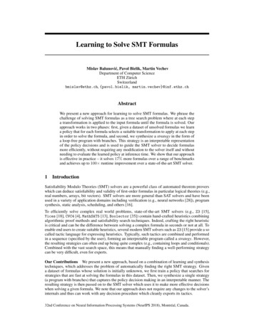
Learning to Solve SMT FormulasMislav Balunović, Pavol Bielik, Martin VechevDepartment of Computer ScienceETH ZürichSwitzerlandbmislav@ethz.ch, {pavol.bielik, martin.vechev}@inf.ethz.chAbstractWe present a new approach for learning to solve SMT formulas. We phrase thechallenge of solving SMT formulas as a tree search problem where at each stepa transformation is applied to the input formula until the formula is solved. Ourapproach works in two phases: first, given a dataset of unsolved formulas we learna policy that for each formula selects a suitable transformation to apply at each stepin order to solve the formula, and second, we synthesize a strategy in the form ofa loop-free program with branches. This strategy is an interpretable representationof the policy decisions and is used to guide the SMT solver to decide formulasmore efficiently, without requiring any modification to the solver itself and withoutneeding to evaluate the learned policy at inference time. We show that our approachis effective in practice – it solves 17% more formulas over a range of benchmarksand achieves up to 100 runtime improvement over a state-of-the-art SMT solver.1IntroductionSatisfiability Modulo Theories (SMT) solvers are a powerful class of automated theorem proverswhich can deduce satisfiability and validity of first-order formulas in particular logical theories (e.g.,real numbers, arrays, bit vectors). SMT solvers are more general than SAT solvers and have beenused in a variety of application domains including verification (e.g., neural networks [28]), programsynthesis, static analysis, scheduling, and others [16].To efficiently solve complex real world problems, state-of-the-art SMT solvers (e.g., Z3 [15],Yices [18], CVC4 [4], MathSAT5 [13], Boolector [35]) contain hand-crafted heuristics combiningalgorithmic proof methods and satisfiability search techniques. Indeed, crafting the right heuristicis critical and can be the difference between solving a complex formula in seconds or not at all. Toenable end users to create suitable heuristics, several modern SMT solvers such as Z3 [15] provide a socalled tactic language for expressing heuristics. Typically, such tactics are combined and performedin a sequence (specified by the user), forming an interpretable program called a strategy. However,the resulting strategies can often end up being quite complex (e.g., containing loops and conditionals).Combined with the vast search space, this means that manually finding a well-performing strategycan be very difficult, even for experts.Our Contributions We present a new approach, based on a combination of learning and synthesistechniques, which addresses the problem of automatically finding the right SMT strategy. Givena dataset of formulas whose solution is initially unknown, we first train a policy that searches forstrategies that are fast at solving the formulas in this dataset. Then, we synthesize a single strategy(a program with branches) that captures the policy decision making in an interpretable manner. Theresulting strategy is then passed on to the SMT solver which uses it to make more effective decisionswhen solving a given formula. We note that our approach does not require any changes to the solver’sinternals and thus can work with any decision procedure which cleanly exports its tactics.32nd Conference on Neural Information Processing Systems (NeurIPS 2018), Montréal, Canada.
We performed an extensive experimental evaluation of our approach on formulas of varying complexity across 3 different theories (QF NRA, QF BV and QF NIA). We show that our synthesized strategiessolve 17% more formulas and are up to 100 faster when compared to the default strategy used inthe state-of-the-art Z3 solver. Further, our learned strategies generalize well and can solve formulaswhich are much more challenging than those seen during training. Finally, we make our tool, calledfastSMT, datasets and experiments available at http://fastsmt.ethz.ch/.2Related workGiven the importance and wide range of SMT solver applications, a number of approaches have beendeveloped to improve both, their runtime as well as the range of formulas they can solve.Portfolio based approaches The most common approach of tools such as SATzilla [44],CPhydra [12], SUNNY [2], Proteus [22], ISAC [27] is a portfolio based method. The key ideais that different SMT solvers use different heuristics and hence work well for different types offormulas. Then, given several SMT solvers and a dataset of formulas, the goal is to learn a classifierwhich uses features extracted from the given formula to select the right SMT solver (or alternativelydefines order in which to run the solvers). In comparison, we address a harder problem - learn how toinstantiate an SMT solver with a strategy that efficiently solves the given dataset of formulas.Evolutionary search The work most closely related to ours is StratEVO [39] which also studiesthe task of generating SMT strategies. However, StratEVO has several limitations – it performssearch using an evolutionary algorithm which does not incorporate any form of learning, the searchdoes not depend on the actual formula, and local mutations tend to get stuck in local minima (as weshow in our experiments in Section 5). As a result, for many tasks where the suitable strategy cannotbe trivially found (e.g., is very short) their approach reduces to random search. Instead, we leveragemodels that learn from previously explored strategies as well as the current formula. As we show, thisenables discovery of complex strategies that are out of reach for approaches not based on learning.Learning branching heuristics and premise selection Recently, learning techniques have beenapplied to improving performance of SAT solvers [32, 42], constraint programming solvers [34],solving quantified boolean formulas [41], solving mixed integer programming problems [29] aswell as premise selection in interactive theorem provers [1, 43, 33]. At a high level, these arecomplementary to us – we learn to search across many tactics and combine them into high levelstrategies while they optimize a single tactic (e.g., by learning which variable to branch on in SAT).Our work also supports formulas from a wide range of theories (as long as there is a correspondingtactic language) where selecting a suitable high level strategy leads to higher speedups comparedto optimizing a single tactic in isolation. However, there are also common challenges such asdefining a suitable formula representation. This representation can range from a set of hand-craftedfeatures [32, 36], to recursive and convolutional neural networks [33, 1], to graph embeddings [43].We extend this line of work by considering fast to compute representations based on bag of words,syntactic features, and features extracted from a graph representation of the formula.Parameter tuning Finally, a number of approaches exist for finding good parameter configurationsfrom a vast space of both discrete and continuous parameters, including ParamILS [25], GGA [3],TB SPO [24] or SMAC [23]. An interesting application of such approaches to the domain of SAT/SMTsolvers is proposed by SATenstein [30] which first designs a highly parameterized solver frameworkto be subsequently optimized by off-the shelf tools. Although such tools are not applicable for thetask of searching for strategy programs (that include loops and conditionals) considered in our work,they can be used to fine-tune the strategy parameters once a candidate strategy is found.3SMT strategies: preliminariesAt a high level, an SMT solver takes as input a first-order logical formula and then tries to decide ifthe formula is satisfiable. In the process, solvers employ various heuristics that first transform theinput formula into a suitable representation and then use search procedures to check for satisfiability.Existing heuristics include: simplify which applies basic simplification rules such as constant2
Table 1: Formalization of the Strategy language used to express SMT strategies in Z3 [15].(Strategy)q:: tpexprcprobe ./paramparams :: :: :: :: :: :: :: t q; q if p then q else q q else q repeat q, c try q for c using t with paramsTactics { bit blast, solve eqs, elim uncnstr . . . }p p p p expr ./ exprc probe expr exprConsts QProbe Q, Probe { num consts, is pb, . . . } / 6(Param, Q), Param { hoist mul, flat, som, . . . } param; paramsfolding (x 0 x), removal of redundant expressions (x x 0), gaussian elim whicheliminates variables (x 1 y x z y 1 z) using Gaussian elimination, elim term itewhich replaces the term if-then-else with fresh auxiliary declarations (if x y then x else y) z k z (x y k x) (x y k y), or bit blast which reduces bit-vectorexpressions by introducing fresh variables, one for each bit of the original bit-vector (e.g., a bitvector of size 4 is expanded into four fresh variables). In total, the Z3 SMT solver defines more than100 such heuristic transformations (called tactics) that can be combined together to define a customstrategy. For example, a strategy for integer arithmetic can be defined as1 :using simplify with (som : true); normalize bounds; lia2pb; pb2bv; bit blast; satAlthough the above sequence of transformations (tactics) works well for some types of input formulas(e.g., in case every variable has a lower and an upper bound), for other formulas a different set oftactics is more suited. In some cases, the suitable set of tactics can be obtained by a small modificationof the original tactic while in others, a completely different set of tactics needs to be defined. As aconcrete example, consider the following strategy implemented in the Yices SMT solver [18, 17]:num atoms k) then simplex else floyd warshallif ( diff dimHere, two high level tactics can be applied to solve an input formula – the Simplex algorithm orthe algorithm based on Floyd-Warshall all-pairs shortest distance. The Simplex algorithm is usedif the input formula is not in the difference logic fragment (denoted using diff) and the ratio ofinequalities divided by the number of uninterpreted constants is smaller than a threshold k.Language for expressing SMT solver strategies In Fig. 1 we formalize the language used byZ3 to enable control over the core solver heuristics. The basic building blocks of the languageare called tactics and represent various heuristic transformations that might be applied during thesearch. Optionally, each tactic can define a set of parameters that affect its behavior. For example, thesimplify tactic contains 50 different parameters that control which simplifications are performed(e.g., if som : true then simplify puts polynomials in som-of-monomials form). The tactics arecombined into larger programs either sequentially or using one of the following control structures: if p then q1 else q2 : If the predicate p evaluates to true apply q1 , otherwise apply q2 .The predicate can contain arithmetic expressions as well as Probes which collect statisticsof the current formula (e.g., num consts returns the number of non-boolean constants). q1 else q2 : First apply q1 and if it fails then apply q2 on the original input. repeat q, c: Keep applying q until it does not modify the input formula any more or thenumber of iterations is greater than the constant c. try q for c: Apply q to the input and if it does not return in c millisenconds then fail. using t with params: Apply the given tactic t with the given parameters params.1For more information and examples we refer the reader to the online tutorial available at:https://rise4fun.com/z3/tutorial/strategies3
4Learning SMT strategiesWe now present our approach for synthesizing SMT strategies. Formally, the task we are interested insolving is defined as follows:Problem statement Given a dataset of SMT formulas F {fi }Ni 1 , our goal is to find a strategy:qbest arg minq StrategyNXdefcost(fi , q) where cost(fi , q) i 1 runtime(q(fi ))if q solves fi(1)timeout penalty otherwiseHere, runtime(q(fi )) Q denotes the runtime required for strategy q to solve formula fi andtimeout penalty Q is a constant denoting the penalty for not solving fi (either due to timeoutor because the strategy q is not powerful enough). Our goal is to find a strategy that minimizes thetime required to solve the formulas in the dataset F. Note that our cost function reflects the fact thatwe aim to synthesize a strategy that solves as many formulas as possible yet one that is also the fastest.Generally, optimizing for Equation 1 directly is problematic as using runtime makes the optimizationproblem inherently noisy and non-deterministic. It also makes learning hard to parallelize due tosignificant impact of hardware and environment on overall runtime. Thus, instead of runtime, we usethe amount of work measured as the number of basic operations performed by the solver required tosolve a formula (e.g., implemented via the rlimit counter in Z3).Challenges To solve the problem of learning SMT strategies, one has to address two challenges: Interpretability. We are interested in learning a model that is not only efficient at solvinga given set of formulas but also expressible as programs in the Strategy language. This isimportant as the learned strategies can then be directly used an input to existing solvers. No prior domain knowledge. Our learning does not assume any prior knowledge aboutthe dataset F and which strategies work best in general – initially the solution to all theformulas in the dataset is unknown, no existing strategies are used to boostrap the learning(not even the default strategies already written by the SMT solver developers) and we donot rely on any heuristics (and their combination) that may be useful in solving formulasfrom F. Indeed, this represents the most challenging setting for learning.Our approach The key idea behind learning a program qbest Strategy efficiently is to takeadvantage of the fact that each program q can be decomposed into a set of smaller branch-freeprograms q1,.,k , each qi corresponding to one execution path of q. This is possible because programsin the Stategy language do not contain state (all state is implicitly captured in the formula beingsolved). As a result, in our approach we learn a program qbest Strategy via a two step process: Learn candidate strategies. First, we learn a policy which finds a set of candidate strategiesconsisting of only sequences of tactics where each strategy performs well on a differentsubset of the dataset F. This allows us to phrase the learning problem as a tree search overtactics for which state-of-the-art models can be used. This step is described in Section 4.1. Synthesize a combined strategy. Then, given a set of candidate strategies, we combine theseinto a single best strategy qbest by synthesizing control structures such as branches and loopsas supported by the Strategy language. This step is described in Section 4.2.4.1Learning candidate strategiesWe phrase the problem of learning candidate strategies as a tree search problem. We start from aninitial state s0 and at each timestep t we choose an action at that expands the tree by exploringa single edge. In our setting, a state corresponds to a tuple consisting of an SMT formula anda strategy used to compute the formula. An action is described by a tactic and its parameters (if any)a Tactics Params. Applying an action transforms the formula into another one. Terminalstates are those that decide the initial formula f , that is, f was reduced to a form that is either triviallysatisfiable or unsatisfiable. Further, for practical reasons, terminal states also include those to whichapplying an action (tactic) leads to a timeout.4
eval. on fEmbeddingTactics0.70 : pb2bv0.15 : smt0.01 : sat.Sigmoid[1733, 0, . . . ]ReLUFormula RepresentationBOW Skip-Gram ASTeval. on fReLUZ3 Probes[num consts, is pb, . . . ]SoftMaxEmbedding[simplify, sat, PAD, . . . ]ReLUStrategyParams0.20 : flat0.75 : som0.95 : factor.Figure 1: Architecture of the neural network model which predicts next tactic and arguments.A terminal state defines a strategy q (i.e., a sequence of tactics starting from the tree root) withan associated cost(f, q) (as defined in Equation 1) that we aim to minimize. During the searchwe keep a priority queue of tuples (s, a, p) consisting of a state, possible action and its associatedprobability, initialized with (s0 , , 1). At each step, we remove the tuple with highest probabilityfrom the queue, apply its action to obtain a new state si and update the priority queue with new tuples(si , a, p · π(a si )) for all actions a Tactics Params capturing the possible transitions from si .Our goal is to learn a policy, denoted as π(a s), that represents a probability distribution of actionsconditioned on a state s. Ideally, the learned distribution should be such that selecting the most likelyaction at that state minimizes the expected cost. In what follows we first describe the models used torepresent the policy π considered in our work and then describe how the models are trained, includinghow to construct a suitable training dataset.Bilinear model Based on matrix factor models used in unsupervised learning of word embeddings[11, 38] as well as supervised text classification [26] we define a bilinear model as follows:π(a s) σ(U V φ(s, a))where φ(s, a) is a bag of features computed for action a taken in state s, U Rk h and V Rh V are the learnable weight matrices, V is the input vocabulary and σ is softmax computing the probabilitydistribution over output classes (in our case actions to be taken in a given state s). As the set of allpossible actions is too large to consider, we randomly generate a subset of parameters for each tacticbefore training starts, thus obtaining the overall set of actions S Tactics Params. We defineφ(s, a) to be all n-grams constructed from the strategy of state s. For example, for strategy a1 ; a2 ; a3 ,the extracted n-grams (features) are described by the vector: ha1 , a2 , a3 , a1 a2 , a2 a3 , a1 a2 a3 i. Then,the vocabulary set V is simply the collection of all possible n-grams formed over S.Neural network Our second model is based on a neural network and improves over the bilinearmodel in two key aspects – it considers a richer state when making the predictions and predicts tacticsas well as their corresponding parameters. The architecture of the neural network model is illustratedin Fig. 1 and uses two inputs: (i) the strategy in the current state (as in the bilinear model), and (ii)the formula f to be solved in the current state. The strategy is encoded by first padding it to beof fixed size, concatenating the embedding of each action in the strategy into a single vector andfinally feeding the resulting vector into a fully-connected layer. We encode the input formula in twoways: first, by computing a set of formula measures such as the number of expressions and constants,and second, by learning a representation of the formula itself. The formula measures are computedusing probes supported by Z3 and are a subset of the possibilities one could define. For the learnedrepresentation of the formula we experimented with three different approaches: Bag-of-words (BOW): The formula is treated as a sequence of tokens from the SMT-LIBlanguage. We obtain its bag-of-words and use it as the formula embedding. Abstract Syntax Tree (AST): From the formulas’s AST, we extract all subtrees of depth atmost two. The bag-of-words over such subtrees is used as the formula embedding. Notethat subtrees which appear in less than 5% of formulas in F are discarded. Skip-gram: Each formula in the dataset is treated as a sequence of tokens over whichwe learn a skip-gram model. We define embedding of the formula as the average of allembeddings of its tokens.5
123456Algorithm 1: Iterative algorithm used to train policy πData: Formulas F, Number of iterations N , Number of formulas to sample K, Explorationrates β, Exploration policy πexplore (e.g., random policy)Result: Trained policy π, Explored strategies QD ; Q ; π policy initializationfor i 1 to N doπ̂ β i π (1 β i )πexplore. policy π̂ explores with probability (1 β i )Q Q Top K most likely strategies for each formula in F according to π̂D D Extract training dataset from strategies Qπ Retrain model π on DThe network output consists of two parts – a probability distribution over tactics to apply next and anassignment to each tactic parameter. The possible tactic parameters are captured by the set Paramfrom Fig. 1. We provide a full list of tactics and their parameters in the extended version of our paper.To compute arguments for the tactic parameters, the network introduces a separate output layer foreach parameter type. The layer performs regression and outputs normalized values in the range [0, 1].For boolean parameters, values 1 and 0 correspond to true and false, respectively. For integerparameters, the output of the network is mapped and discretized into the range of allowed values.Model training At a high level, our training is based on the DAgger method [40] and is shown inAlgorithm 1. The training starts with a randomly initialized policy used to sample the top K mostlikely strategies for each formula in the training dataset F (line 4). Selected strategies are evaluatedand used to create a training dataset (line 5, described below) on which the policy π is retrained(line 6). As the model is initially untrained the strategies are sampled at random and only as thetraining progresses the policy will learn to select strategies that perform well on formulas from F. Asan alternative, one could pre-train the initial policy using strategies supplied by an expert in whichcase the algorithm would correspond to imitation learning. However, in our work we assume suchexpert strategies are not available and therefore we start with a model that is initialized randomly.Building the training dataset Each sample in our training dataset D {h(ti , pi ), si i}Mi 1 for theneural network consists of a state and its associated training label. Here, the label is a tuple consistingof a probability distribution over tactics t R Tactics and the values of all tactic parametersp R Param . The intuition behind this choice is that for a state s, the vector t encodes the likelihoodthat a given tactic is fast at solving the formula whereas p contains the best parameter values foundso far during training. Generating the dataset in this way encodes the preference for strategies thatare most efficient in contrast to finding any strategy that solves the input formula. To train the neuralnetwork model using such a dataset, the loss is constructed as a weighted average of the cross-entropyloss for tactic prediction and mean-squared-error for parameter prediction.We build the dataset as follows. First, we evaluate each strategy in Q on the formula for which itwas generated and keep only those that succeeded in deciding the formula. Second, let us denotewith r(t, si ) the best runtime (or timeout) achieved from state si by first applying tactic t, withrbest (si ) the best runtime achieved from state si , and with v(p, si ) the value assigned to parameter pin tactics with the best runtime from state si . We obtain r, rbest and v by considering all the statesand actions performed when evaluating the strategies in Q. Then, for each non-terminal state si thateventually succeeded we create one training sample h(σ(t i ), pi ), si i where t i [1/r(t, si )]t Tactics ,σ normalizes t i to a valid probability distribution and pi [v(p, si )]p Param . To generate thetraining dataset for bilinear model we follow a similar procedure with the exception that we uset i 1[rbest (si ) r(t, si )]t Tactics which assigns probability 1 to the best tactic and 0 to others.Pruning via equivalence classes A challenge in training the models presented above is that whethera strategy solves the formula is known only at terminal states. This is especially problematic fordatasets where majority of the effort is spent on finding any successful strategy. To address thisissue we take advantage of the fact that some information can be learned also from partial strategies– namely their current runtime and their transformed formula. This allows us to check if multipletransformed formulas are equivalent (we consider two formulas equivalent if their abstract syntaxtress are identical) and keep only the one which was fastest to reach (and prune the others).6
a1a2a4a3a5tree representation of q1 and q2q1 a1 ; a2 ; a3q2 a1 ; a4 ; a5f11030f2100TIMEOUTf310020formulas f1 , f2 , f3 and their associated costsf1f2f3200 250 30num exprformula measurebranch with cost 0.276 ( 1/3 · log(1/3) 2/3 · log(2/3)) 0if true then a2 elseif num expr 100 then a2 else a4branch with cost 0.2 2/3 · log(1/2) 1/3 · 0Figure 2: Illustration of decision tree representation of strategies, scored formulas and branches.4.2Synthesizing a combined, interpretable strategyThe policy π learned in Section 4.1 can be used to speed-up SMT solving as follows: invoke thesolver with the current formula f and the action a0 selected by π, obtain a new intermediate formulaf1 from the solver, then again invoke the solver from scratch with f1 and a new action a1 , obtaininganother intermediate formula f2 , and so on. Unfortunately, even if the final formula fk is solved (e.g.,determined to be SAT), we would have lost the connection with the original formula f as at eachstep we are making a new, fresh invocation of the SMT solver. This is problematic for tasks (e.g.,planning) that require more information from SMT solvers, beyond satisfiability of f , for instance,the model itself. To address this challenge without changing the internals of the SMT solver, wepropose to synthesize an interpretable policy qbest that follows π and can be directly expressed in theStrategy language from Fig. 1 (and thus be given as input to the SMT solver).Recall from Fig. 1 that the Strategy language defines two types of statements that can be used tocombine programs: if-then-else and or-else. However, notice that the or-else statement is infact a special version of the if statement with a condition that checks if a given tactic terminateswithin c milliseconds. As a result, we can reduce the problem of synthesizing programs in theStrategy language to the problem of synthesizing branches with predicates over a set of candidatestrategies. We can obtain the set of candidate strategies by either evaluating π over the trainingformulas or by extracting successful strategies from the set Q explored during policy learning. Next,we discuss how to synthesize qbest .Decision tree learning To synthesize branches with predicates, we adapt techniques based ondecision tree learning. Consider the tree illustrated in Fig. 2 (top left) with the same structure asused during search (i.e., edges denoting actions and nodes denoting states) but formed from thetwo candidate strategies q1 and q2 . Each SMT formula is evaluated by taking a path in the tree andapplying all the corresponding actions. Intuitively, at each node with more than one outgoing edgea decision needs to be taken to determine which path to take. To encode such decisions, our goal is tointroduce one or more branches at each such node (denoted as orange square in Fig. 2).More formally, let Q {q1 , . . . , qn } be a set of candidate strategies, F be our dataset of formulasand b :: if p then q true else q false a branch that partitions F into two parts – Ftrue are formulason which predicate p evaluates to true and Ffalse for the rest. We define a notion of multi-labelentropy of a dataset of formulas, denoted as H(F) [14]:XH(F) p(q) log(p(q)) (1 p(q)) log(1 p(q))q Qwhere p(q) denotes the ratio of formulas solved by strategy q in F. The goal of synthesis is then todiscover branches that partition F into smaller sets, each of which has small entropy (i.e. either noneor all formulas are solved). Using the entropy, we define a cost associated with a branch b as:cost(b, Ftrue , Ffalse ) ( Ftrue / F )H(Ftrue ) ( Ffalse / F )H(Ffalse )That is, branch cost is a weighted sum of entropies in each of the resulting branches. With this scoringfunction we build the decision tree in a top-down fashion – for each node with multiple outgoingedges we recursively synthesize predicates that minimize the cost. If dataset size for some node isbelow a certain threshold we greedily select the strategy which can solve the most formulas, breakingties using runtimes. To express branches, we consider the following types of predicates: (i) truewhich allows expressing a default choice, (ii) Probes with arithmetic expression as defined in Fig. 1,and (iii) try s for c which allows checking whether tactics terminate within c ms.7
Models ComparisonEffect of State egy0.8PerformancePerformance0.80.6 Probes BOWProbes Skip-gramProbes ASTProbes0.40.20204060800.0100Number of sampled strategies01020304050Number of sampled strategiesFigure 3: Comparison of proposed models and baselines for learning SMT solver strategies. Each line(higher is better) denotes the quality of the best learned strategy among top x most likely strategiesfound by a given model (x axis) proportional to the best known strategy overall (y axis).5ExperimentsWe implemented our method in a system called fastSMT and evaluated its effectiveness on 5 differentdatasets – AProVE [19, 5], hycomp [7], core [6], leipzig [8] and Sage2 [9, 21]. These containformulas of varying complexity across 3 logi
Learning to Solve SMT Formulas Mislav Balunovic, Pavol Bielik, Martin Vechev Department of Computer Science ETH Zürich Switzerland bmislav@ethz.ch, {pavol.bielik, martin.vechev}@inf.ethz.ch Abstract We present a new approach for learning to solve SMT formulas. We phrase the challenge of solving SMT formulas as a tree search problem where at .